1 Intro

**Figure** 1: VCF Eurorack module (left) and VCV Model (right)

In this post we’ll be continuing to reproduce the designs of the mki x es.edu eurorack VCF. The detailed build instructions (source: https://www.ericasynths.lv/shop/diy-kits-1/edu-diy-vcf/) contain lots of great information and it’s recommended to read that document first.

This part focuses on adding resonance to RC designs in Part 1.

2 Fixed Resonance

The starting point for adding resonance to the circuit is to simply feed the second filtering stage’s output to the first stage’s capacitor.

def generate_rc_2nd_order_fixed_resonance(Rf=200):
    # RC 2nd order active (with fixed resonance)
    netlist = """
    V0 1 0 Vin
    R 1 2 Rf
    C1 5 2 1.0e-6
    OAmp 2 3 3
    R 3 4 Rf
    C2 4 0 1.0e-6
    OAmp 4 5 5
    J 5 0
    """
    class_name = "RCFilter2ndOrderFixedResonance"
    rules, _ = run_MNA(netlist, class_name)
    code_string = generate_processor(rules)

    fig, axs = plt.subplots(2, 1, figsize=(12, 8))

    with ModuleLoader(code_string, class_name) as m:
        tmax, dt = 0.05, 1.0 / 44100.0
        ts = np.arange(0, tmax, dt)
        fn = square(freq=50, ppv=5.0)
        v_ins = fn(ts)
        v_outs = []
        for v_in in v_ins:
            v_outs.append(m.process(v_in, Rf, dt))

        axs[0].set_title("square wave")
        axs[0].plot(ts, v_ins, label="V_in")
        axs[0].plot(ts, v_outs, label="V_out")
        axs[0].legend()

        for i, Rf in enumerate([1000, 3300, 10000]):
            plot_filter_response(
                m,
                ax=axs[1],
                args=(Rf,),
                title="Frequency Response: Resonance",
                label=f"$R_f = {Rf}\Omega$",
            )

            # where we expect the cutoff to be
            cutoff_expected = 1 / (2 * np.pi * Rf * 1e-6)
            axs[1].axvline(cutoff_expected, linestyle=":", color=colors[i])

    axs[1].set_xlim(0.3, 1e3)
    axs[1].set_ylim(-30, 6)
    plt.show()


generate_rc_2nd_order_fixed_resonance()

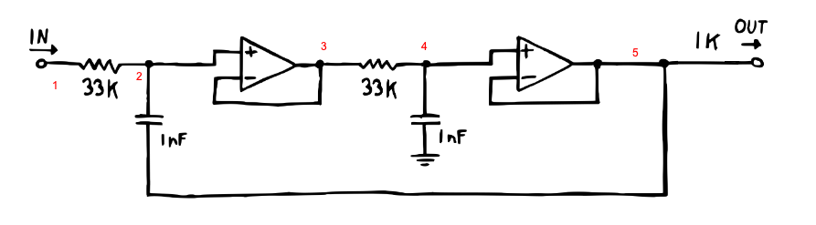
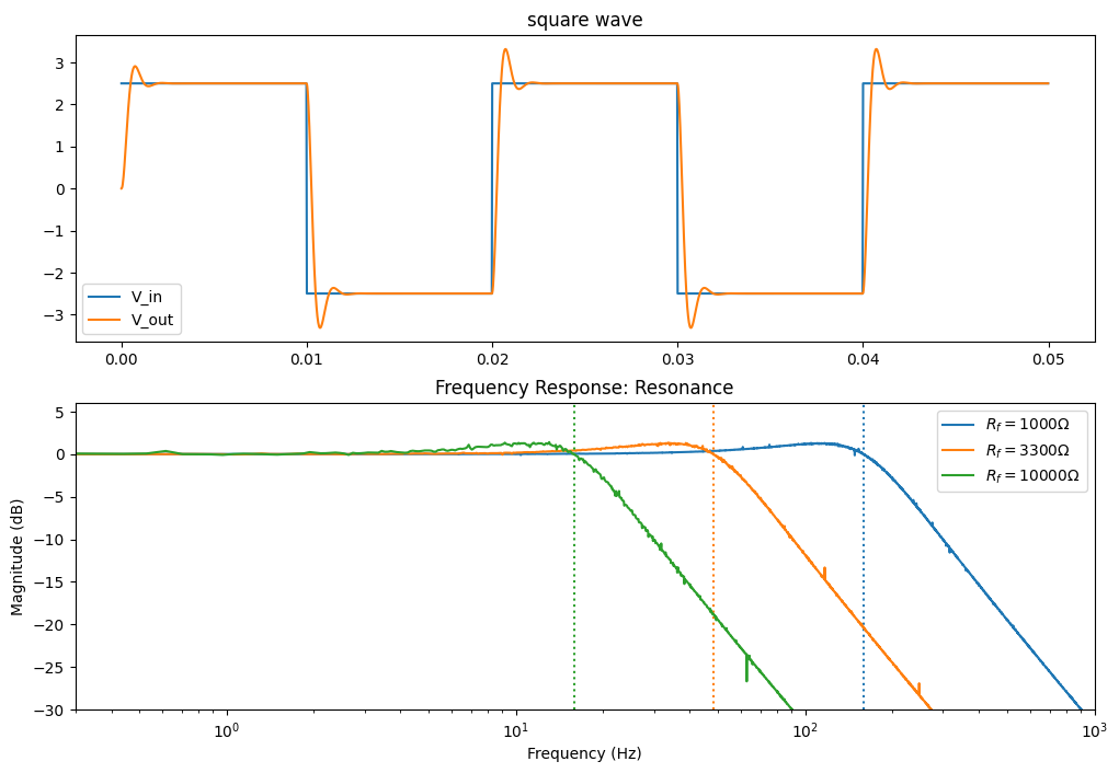
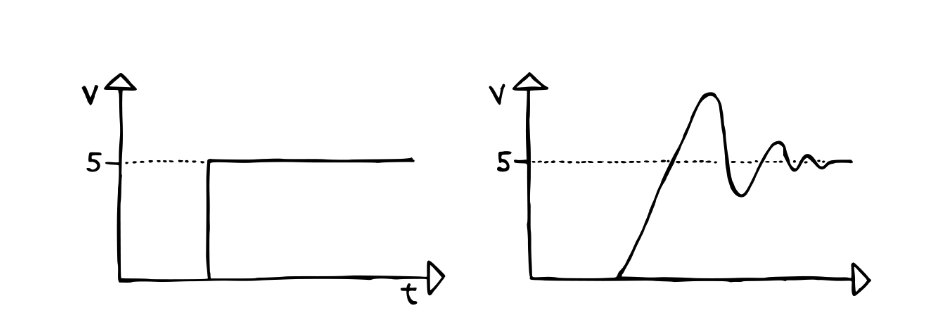
As we can see, the feedback path adds a slight ringing on abrupt changes in the waveform, similar to the schematic that Moritz shows:

**Figure** 3: Schematic of resonance effect on a square wave. Source: Moritz’s guide

Also looking at the frequency spectra, we can see that frequencies near the cutoff frequency are slightly accentuated. Next we see how increase or decrease this effect.

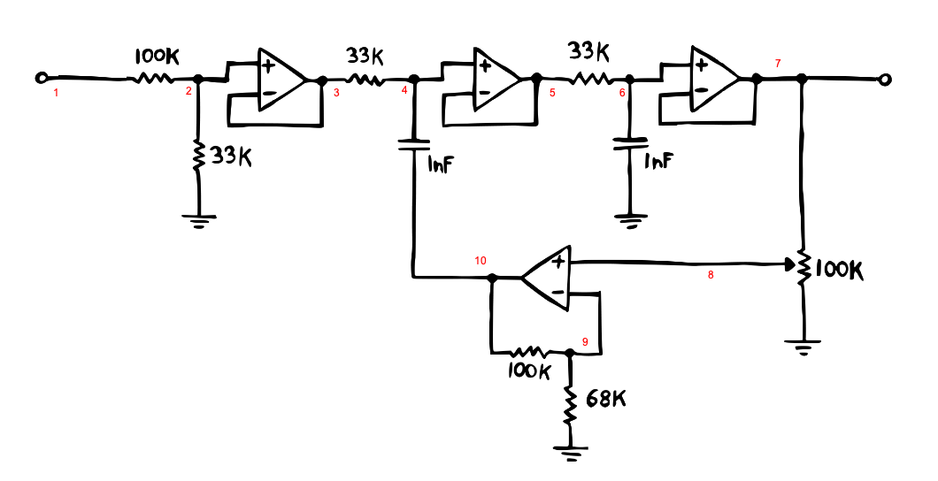
3 Variable Resonance (Ideal OpAmps)

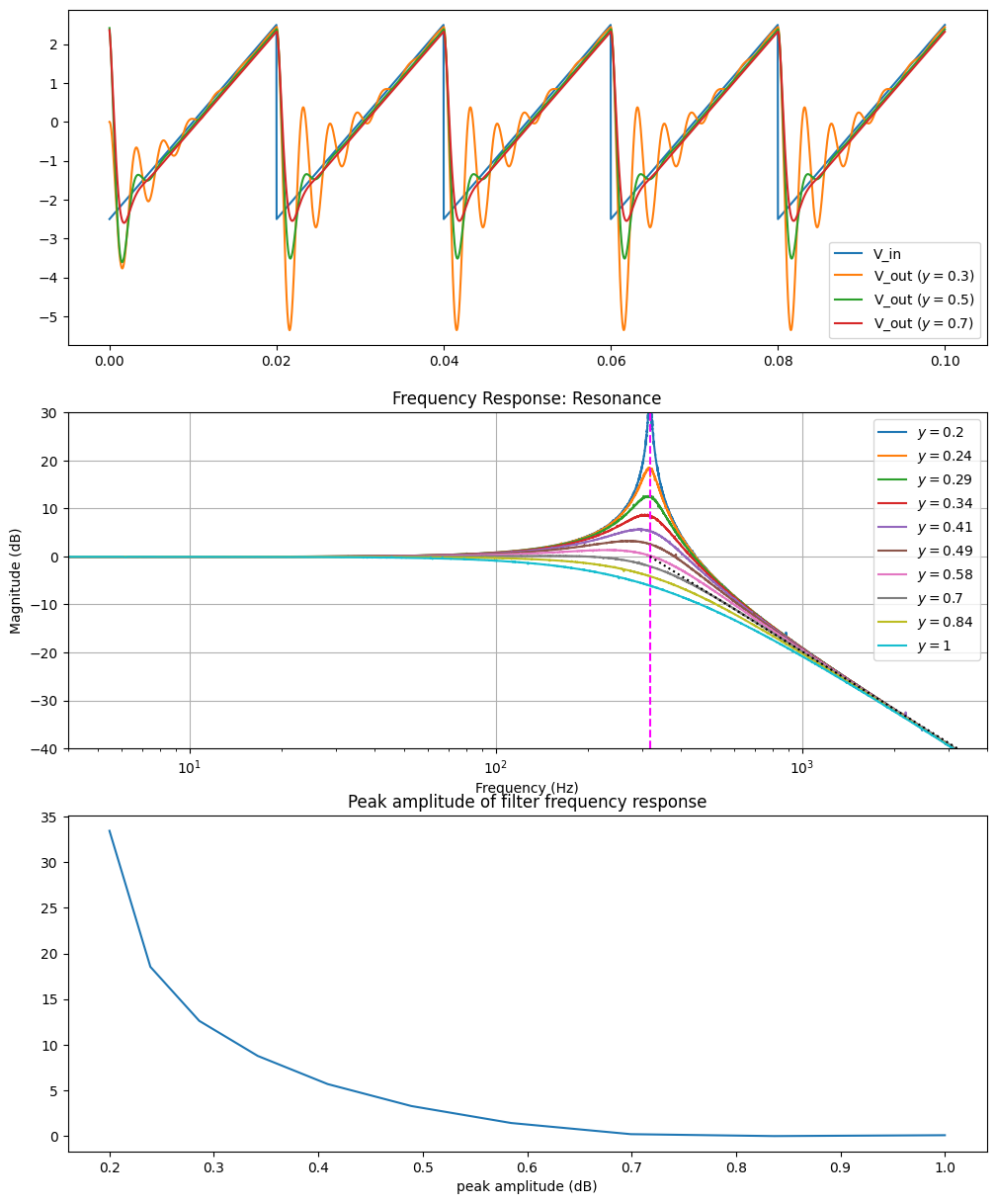
**Figure** 4: Variable resonance, 2nd order

In order to control the level of resonance, we need to scale the filter’s output down before sending it back to the capacitor. Moritz’s design which uses a potentiometer to dynamically control the resonance is shown above. We’ve made one small change which is to bring the gain back up to unity (the design in the manual has a drop in gain of /4).

Note

TODO: check why this isn’t equivalent to removing the initial /4 gain voltage divider.

def generate_rc_2nd_order_variable_resonance(y=0.3):
    # output is node 7
    netlist = """
        V0 1 0 Vin
        R100k 1 2 100000   #voltage divider
        R33k 2 0  33000   #voltage divider
        Oamp 2 3 3
        Rf 3 4  Rf
        Oamp 4 5 5
        Rf 5 6  Rf
        Oamp 6 7 7
        P 7 8 0 100000 # reso amount
        Oamp 8 9 10  
        R68k 9 0   68000
        R100k 9 10 100000
        C1 10 4 1e-6
        C2 6 0 1e-6
        # final stage not in Moritz design, but compensates for /4 drop in amplitude
        Oamp 7 11 12
        Ra 11 0  100
        Rb 11 12 300
        J 12 0
    """

    Rp, R100k = symbols("Rp R100k")
    assumptions = {Rp: R100k}
    class_name = "RCFilter2ndOrderVariableResonance" + str(np.random.randint(100000))
    assignments, _ = run_MNA(
        netlist, class_name, method="linsolve", assumptions=assumptions
    )

    code_string = generate_processor(assignments)

    fig, axs = plt.subplots(3, 1, figsize=(12, 15))

    Rf, y, C = 500.0, 0.3, 1e-6

    # and where we expect the cutoff to be
    cutoff_expected = 1 / (2 * np.pi * Rf * C)

    with ModuleLoader(code_string, class_name) as m:
        tmax, dt = 0.1, 1.0 / 44100.0
        ts = np.arange(0, tmax, dt)
        saw_fn = saw(freq=50, ppv=5.0)
        v_ins = saw_fn(ts)
        axs[0].plot(ts, v_ins, label="V_in")

        for y in [0.3, 0.5, 0.7]:
            v_outs = []
            for v_in in v_ins:
                v_out = m.process(v_in, Rf, y, dt)
                v_outs.append(v_out)

            axs[0].plot(ts, np.array(v_outs), label=f"V_out ($y = {y:.1g}$)")
            axs[0].legend()

        filter_peaks = []
        ys = np.geomspace(0.2, 1.0, 10)
        for y in ys:
            _, H_dB, _, _ = plot_filter_response(
                m,
                ax=axs[1],
                args=(Rf, y),
                title="Frequency Response: Resonance",
                label=f"$y = {y:.2g}$",
            )
            filter_peaks.append(H_dB.max())

        order = 2
        # and where we expect the cutoff to be
        cutoff_expected = 1 / (2 * np.pi * Rf * C)
        axs[1].axvline(cutoff_expected, linestyle="--", color="magenta", label="$f_c$")

        # plot a trendline just for reference, where we expect 12dB / oct for 2nd order
        octaves = 6.5
        axs[1].plot(
            [cutoff_expected, cutoff_expected * (2**octaves)],
            [0, -(octaves * 12)],
            ":",
            color="k",
            label="12dB / oct",
        )

    axs[1].set_xlim(4, 4000)
    axs[1].set_ylim(-40, 30)
    axs[1].grid()

    axs[2].set_title("Peak amplitude of filter frequency response")
    axs[2].plot(ys, filter_peaks)
    axs[2].set_xlabel("y")
    axs[2].set_xlabel("peak amplitude (dB)")
    plt.show()


generate_rc_2nd_order_variable_resonance()

Now the potentiometer controls the strength of the feedback (the fraction of the potentiometer is $y$ ). The peak gain increases with deceasing $y$ . At $y \approx 0.2$ , we can see that the gain is diverging. Running the code at values much below $y = 0.2$ will be numerical unstable, and will quickly produce $V \to inf$ .

4 Variable Resonance (Supply Limited OpAmps)

Of course this doesn’t happen in real hardware, and at a certain point the OpAmp will saturate and not produce higher voltages - this happens at the supply voltage, which would typically be $\pm 12 V$ . Controlling this feedback should allow us to reach the self-oscillation regime.

Note

NOTE: This section is still a WIP as I’m not sure under what numerical conditions self-oscillation “works”. Specifically I only see it when certain OpAmps in the circuit are clamped to $\pm 12 V$ . OpAmps 2 and 3 clamped seems to work, and we use that below.

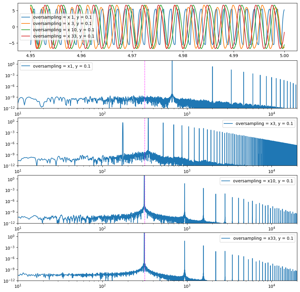
def generate_rc_2nd_order_variable_resonance_clamped(
    ax_t, ax_f, oversampling=1.0, y=0.1, opamps_to_clamp=(2, 3)
):
    clamp_str = {}
    for i in [1, 2, 3]:
        if i in opamps_to_clamp:
            clamp_str[i] = "Vmax=+12"
        else:
            clamp_str[i] = ""

    
    netlist = f"""
        V0 1 0 Vin
        R100k 1 2 100000   #voltage divider
        R33k 2 0  33000   #voltage divider
        Oamp 2 3 3
        Rf 3 4  Rf
        Oamp1 4 5 5 {clamp_str[1]}
        Rf 5 6  Rf
        Oamp2 6 7 7 {clamp_str[2]}
        P 7 8 0 100000 # reso amount
        Oamp3 8 9 10 {clamp_str[3]}
        R68k 9 0   68000
        R100k 9 10 100000
        C1 10 4 1e-6
        C2 6 0 1e-6
        J 7 0              # output
    """

    Rp = symbols("Rp", positive=True)
    R100k = symbols("R100k")
    assumptions = {Rp: R100k}
    class_name = "RCFilter2ndOrderVariableResonanceClamped" + str(
        np.random.randint(100000)
    )
    assignments, _ = run_MNA(
        netlist,
        class_name,
        method="LUsolve",
        assumptions=assumptions,
        simplify_sol=False,
    )

    code_string = generate_processor(assignments)

    Rf, C = 500.0, 1e-6

    # and where we expect the cutoff to be
    cutoff_expected = 1 / (2 * np.pi * Rf * C)

    with ModuleLoader(code_string, class_name) as m:
        tmax, dt = 5, (1.0 / 44100.0) / oversampling
        ts = np.arange(0, tmax, dt)
        v_ins = 0.01 * np.random.normal(size=ts.shape)
        v_ins[0 : len(v_ins) // 10] = 0.0

        v_outs = []
        for v_in in v_ins:
            v_out = m.process(v_in, Rf, y, dt)
            v_outs.append(v_out)

        v_outs = np.array(v_outs)
        ax_t.plot(
            ts[ts > tmax - 0.05],
            v_outs[ts > tmax - 0.05],
            label=f"oversampling = x {oversampling:.3g}, y = {y}",
        )
        ax_t.legend()

        # discard first half of time data (not steady state)
        f, Pyy = periodogram(v_outs[len(v_outs) // 2 :], fs=1.0 / dt, window="flattop")

        ax_f.loglog(f, Pyy, label=f"oversampling = x{oversampling:.3g}, y = {y}")
        ax_f.set_xlim(10, 20000)
        ax_f.set_ylim(1e-12, 10)
        ax_f.axvline(cutoff_expected, linestyle=":", color="magenta")
        ax_f.legend()
    return v_outs


display()

display(
    Markdown(
        "Top plot, time series, lower plots convergence study for increasing level of oversampling."
    )
)

fig, ax = plt.subplots(5, 1, figsize=(12, 12))
generate_rc_2nd_order_variable_resonance_clamped(
    ax_t=ax[0], ax_f=ax[1], oversampling=1.0
)
generate_rc_2nd_order_variable_resonance_clamped(
    ax_t=ax[0], ax_f=ax[2], oversampling=3.0
)
generate_rc_2nd_order_variable_resonance_clamped(
    ax_t=ax[0], ax_f=ax[3], oversampling=10.0
)
generate_rc_2nd_order_variable_resonance_clamped(
    ax_t=ax[0], ax_f=ax[4], oversampling=33.0
)
plt.show()

Top plot, time series, lower plots convergence study for increasing level of oversampling.

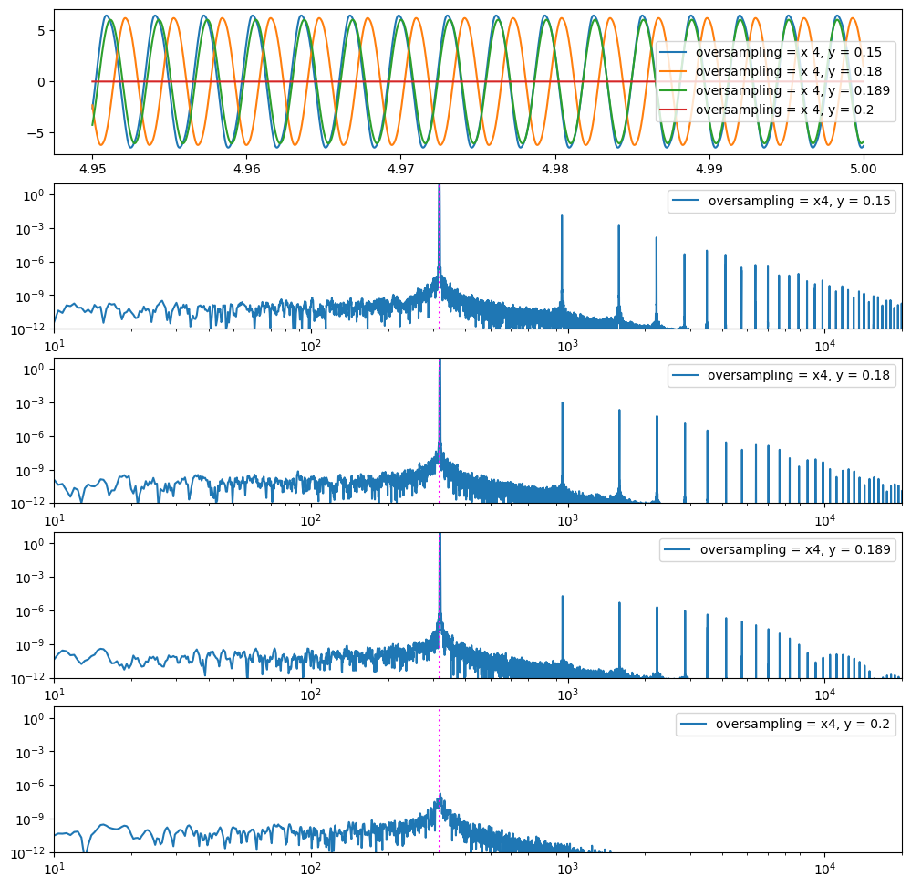
Next we show the transition from self-oscillating (when $y$ is small) to quiescence (for larger $y$ ).

fig, ax = plt.subplots(5, 1, figsize=(12, 12))
generate_rc_2nd_order_variable_resonance_clamped(
    ax_t=ax[0], ax_f=ax[1], oversampling=4, y=0.15
)
generate_rc_2nd_order_variable_resonance_clamped(
    ax_t=ax[0], ax_f=ax[2], oversampling=4, y=0.18
)
generate_rc_2nd_order_variable_resonance_clamped(
    ax_t=ax[0], ax_f=ax[3], oversampling=4, y=0.189
)
generate_rc_2nd_order_variable_resonance_clamped(
    ax_t=ax[0], ax_f=ax[4], oversampling=4, y=0.2
)
plt.show()

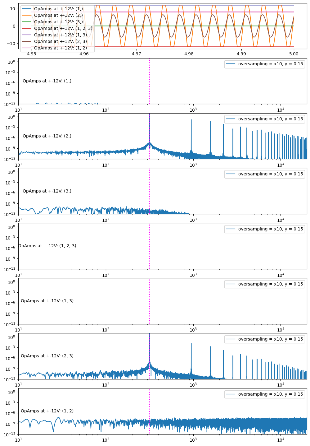
Finally we try to understand why only certain combinations of “clamped” (or non-ideal) OpAmps allow self-oscillation. For certain combinations the voltage just spikes to the rail voltage and gets stuck.

fig, ax = plt.subplots(8, 1, figsize=(12, 18))
labels = []
for i, opamps_to_clamp in enumerate(
    [(1,), (2,), (3,), (1, 2, 3), (1, 3), (2, 3), (1, 2)]
):
    v_outs = generate_rc_2nd_order_variable_resonance_clamped(
        ax_t=ax[0],
        ax_f=ax[1 + i],
        y=0.15,
        oversampling=10.0,
        opamps_to_clamp=opamps_to_clamp,
    )

    print(
        f"clamped: {opamps_to_clamp}, {np.isinf(v_outs).any() or np.isnan(v_outs).any()}, {np.abs(v_outs).max()}"
    )

    ax[1 + i].text(
        0.1,
        0.5,
        f"OpAmps at +-12V: {opamps_to_clamp}",
        horizontalalignment="center",
        verticalalignment="center",
        transform=ax[1 + i].transAxes,
    )

    labels.append(f"OpAmps at +-12V: {opamps_to_clamp}")
ax[0].legend(labels=labels)
plt.show()

clamped: (1,), False, 11.999913215637207
clamped: (2,), False, 11.999638557434082
clamped: (3,), False, 4.673670768737793
clamped: (1, 2, 3), False, 11.987473487854004
clamped: (1, 3), False, 11.999423027038574
clamped: (2, 3), False, 6.475559234619141
clamped: (1, 2), False, 12.000199317932129

/var/folders/m2/93knd1zj1d5f239y0mm3x7280000gn/T/ipykernel_75742/3038351426.py:74: UserWarning: Data has no positive values, and therefore cannot be log-scaled.
  ax_f.set_xlim(10, 20000)