
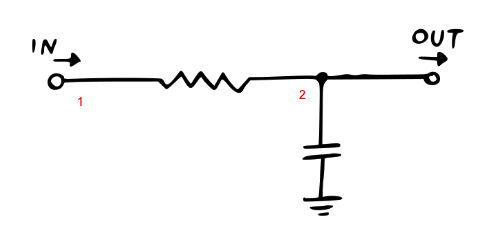
netlist = """
V0 1 0 Vin
R 1 2 R
C 0 2 1.0e-6
J 2 0
"""
circuit_name = "RCFilter1stOrder"
circuit = parse_netlist(netlist, circuit_name)
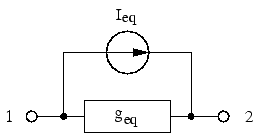
ieq, gc, cieq, cgc, v_2 = symbols("i_eq, g_c, c.ieq, c.gc, v_2")
assumptions = {cieq: ieq, cgc: gc}
(A, x, b), solutions, _ = solve_for_unknown_voltages_currents(
circuit, assumptions=assumptions
)
display(Eq(MatMul(A, x), b))
display(Eq(Mul(A, x), b))1 Intro
In this post we’ll be working to reproduce the mki x es.edu eurorack VCF. The detailed build instructions (source: https://www.ericasynths.lv/shop/diy-kits-1/edu-diy-vcf/) contain lots of great information and it’s recommended to read that document first.
This part focuses on the simplest designs, the RC filters - later sections will consider topics such as resonance and diode ladders.
2 Maths diversion: modelling capacitors
Until this point, we’ve only considered time-independent components, e.g. resistors, op-amps, diodes. Capacitors, an essential component of the filter, are time-dependent, i.e. they have some state that depends on the previous history of voltages across the device. The current through a capacitor can be expressed as:
where
So given a solution for the voltage at time
If we identify
i.e. the current through the capacitor is the series sum of 1) a current source
We already know how to add current sources and resistances to the modified nodal analysis equations, so we can just do the following:
Note that we can substitute in a previously calculated value of
So in summary, when using the trapezoidal approximation, capacitors contribute a constant term
3 Passive RC Filter, 1st order
With the ability to simulate capacitors, we are ready to tackle the most basic filter design, the Passive RC Filter. The basic idea is similar to a voltage divider, except the capacitor can be considered a “frequency dependent resistor.” When the voltage is high and constant, the capacitor charges and the effective resistance gradually increases towards infinity:
When the voltage suddenly drops, the capacitor discharges through the resistor. When the input voltage changes rapidly, the capacitor does not have enough time to fully charge or discharge, and the output signal won’t accurately reflect the input signal, and will be “rounded off” or filtered, examples below.
v_out_update = Assignment(v_2, solutions[v_2])
cap_update = Assignment(ieq, -(2 * gc * v_2 + ieq))

display(Eq(v_out_update.lhs, v_out_update.rhs))
display(Eq(cap_update.lhs, cap_update.rhs))While in general we’ll use SPICEWORLD’s C++ code generation, we can show the principle for this simple example in python. The sympy command pycode will generate python expressions for the above two update rules. So we just need to iterate over time feeding in an input signal to
rc_test_code = f"""
def solve_rc_filter_passive_1st_order(R = 1000, C = 1e-6, wave=square):
    # R - resistor value (Ohms)
    # C - capacitor value (Farads)

    h = 1.0/44100.   # timestep
    t_max = 0.04     # max time
    g_c = 2 * C / h  # capacitor equivelent source conductance

    i_eq = 0
    ts = np.arange(0, t_max, h)
    wave_fn = wave(freq=100, ppv=5.)
    v_ins = wave_fn(ts)

    v_outs = []
    for Vin in v_ins:
        {pycode(v_out_update)}
        {pycode(cap_update)}

        v_outs.append(v_2)

    return ts, v_ins, v_outs
"""
# exec will define the solver
exec(rc_test_code)

# print the code for reference
print(rc_test_code)

for wave in [square, saw]:
    # run it
    ts, v_ins, v_outs_1eneg7 = solve_rc_filter_passive_1st_order(
        R=100, C=1e-6, wave=wave
    )
    ts, v_ins, v_outs_1eneg6 = solve_rc_filter_passive_1st_order(
        R=1000, C=1e-6, wave=wave
    )
    ts, v_ins, v_outs_1eneg5 = solve_rc_filter_passive_1st_order(
        R=10000, C=1e-6, wave=wave
    )

    plt.figure(figsize=(10, 5))
    plt.title(f"Wave: {wave.__name__}")
    plt.plot(ts, v_ins, label="V_in (100 Hz)")
    plt.plot(
        ts,
        v_outs_1eneg5,
        label=f"V_out (R = 100Ω, f_c = {1/(2*np.pi*100*1e-6):.4g} Hz)",
    )
    plt.plot(
        ts,
        v_outs_1eneg6,
        label=f"V_out (R = 1000Ω, f_c = {1/(2*np.pi*1000*1e-6):.4g} Hz)",
    )
    plt.plot(
        ts,
        v_outs_1eneg7,
        label=f"V_out (R = 10000Ω, f_c = {1/(2*np.pi*10000*1e-6):.4g} Hz)",
    )

    plt.xlabel("time")
    plt.legend()
    plt.show()
def solve_rc_filter_passive_1st_order(R = 1000, C = 1e-6, wave=square):
    # R - resistor value (Ohms)
    # C - capacitor value (Farads)

    h = 1.0/44100.   # timestep
    t_max = 0.04     # max time
    g_c = 2 * C / h  # capacitor equivelent source conductance

    i_eq = 0
    ts = np.arange(0, t_max, h)
    wave_fn = wave(freq=100, ppv=5.)
    v_ins = wave_fn(ts)

    v_outs = []
    for Vin in v_ins:
        v_2 = (-R*i_eq + Vin)/(R*g_c + 1)
        i_eq = -2*g_c*v_2 - i_eq

        v_outs.append(v_2)

    return ts, v_ins, v_outs
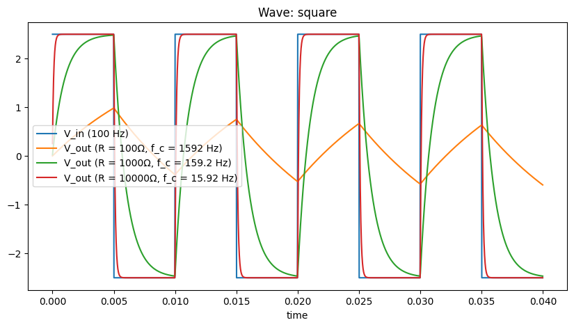
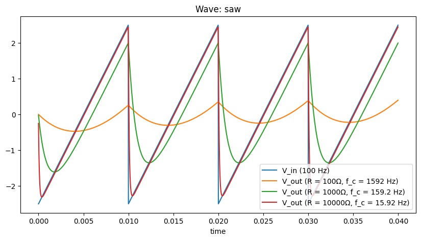
As we can see, depending on the resistor values, the degree to which the input wave (square or saw) is affected varies. Larger resistances (at fixed capacitance) closes off the low pass filter (lower cutoff frequency
Qualitatively the waves become rounded off more and should sound less bright. A more quantitative way to describe the sound is by plotting frequency specta. For this we will use the libraries C++ code generation method generate_processor instead of the ad-hoc python code of the previous section. This simplifies things, e.g., by using classes to track states for the more complex elements (capacitors).
3.1 Frequency Analysis
We would like to plot the filter behaviour as attenuation as a function of frequency - to do this we need to estimate the transfer function.
3.1.1 Theoretical Analysis
If we had a theoretical filter, and we knew the filter coefficients, then we could analytically write down the transfer function. E.g. for the 1st order passive RC, the transfer function reads:
where
We can also think about the “phase” behaviour of a filter. As the RC filter contains a capacitor, output signal ends up lagging behind the input by a phase angle,
3.1.2 Simulation analysis
However we may not in general know the transfer function, e.g. for our circuit models. In this case we can probe it by feeding in white noise (which contains signals at all frequencies and measuring the response. Then we can take the Fourier transform of the output and input and take the ratio to get the transfer function:
We can see why noise is a good signal to probe the filter (though others, e.g. sine sweep are possible) - the transfer function
The scipy library provides csd function that returns the cross spectral density, so we can calculate the gain and phase for input x and output y as follows:
f, csd_xy = csd(x, y, fs=44100., window='flattop', noverlap=0, nperseg=len(v_ins))
f, csd_xx = csd(x, x, fs=44100., window='flattop', noverlap=0, nperseg=len(v_ins))
f, csd_yy = csd(y, y, fs=44100., window='flattop', noverlap=0, nperseg=len(v_ins))

# Compute the frequency response of the filter
H = np.sqrt(csd_yy / csd_xx)
H_mag = 20 * np.log10(H)

# Compute the phase response of the filter
phi = np.angle(csd_xy)
phi = np.unwrap(phi)
phi_deg = np.rad2deg(phi)
Code
def frequency_response_1st_order():
    Rf = 1000
    C = 1e-6
    RC = Rf * C
    fc = 1.0 / (2 * np.pi * RC)

    netlist = f"""
    V0 1 0 Vin
    R 1 2 Rf
    C1 0 2 {C}
    J 2 0
    """
    class_name = "RCFilter1stOrderPassive"
    rules, _ = run_MNA(netlist, class_name)

    code_string = generate_processor(rules)

    fig, axs = plt.subplots(2, 1, figsize=(10, 8))
    with ModuleLoader(code_string, class_name) as m:
        plot_bode(m, axs=axs, args=(Rf,), label="simulated")
        m.reset()

        Rf, tmax, dt = 1000, 0.04, 1.0 / 44100.0
        ts = np.arange(0, tmax, dt)
        # feed in a sin wave at cutoff frequency
        v_ins = np.sin(2 * np.pi * ts * fc)
        v_outs = []
        for v_in in v_ins:
            v_out = m.process(v_in, Rf, dt)
            v_outs.append(v_out)

    f = np.arange(0.01, 22050, 1)

    gain = 1.0 / np.sqrt(1 + np.power(f / fc, 2))
    gain = 1.0 / np.sqrt(1 + np.power(f * 2 * np.pi * RC, 2))
    gain = 20 * np.log10(gain)
    axs[0].semilogx(f, gain, "--", label="analytical")

    # plot the -3dB line
    axs[0].axhline(-3, linestyle="-.", color="black", label="-3dB level")
    # and where we expect the cutoff to be
    cutoff_expected = 1 / (2 * np.pi * Rf * C)
    axs[0].axvline(cutoff_expected, linestyle="--", color="magenta", label="$f_c$")
    axs[0].set_ylim(-50, 6)
    axs[0].legend()

    phase_shift = -np.arctan(f / fc) * 180 / np.pi
    axs[1].semilogx(f, phase_shift, "--", label="analytical")
    axs[1].axvline(fc, linestyle="--", color="magenta", label="$f_c$")
    axs[1].axhline(-45, linestyle="-.", color="black", label="-45 degree phase shift")
    axs[1].legend()
    plt.tight_layout()
    plt.show()

    v_outs = np.array(v_outs)
    fig, ax = plt.subplots(figsize=(10, 5))
    ax.plot(ts, v_ins, label="V_in")
    ax.plot(ts, v_outs, label="V_out")
    ax.set_xlim(0.035, 0.040)
    ax.set_xlabel("t")
    ax.legend()
    plt.show()


frequency_response_1st_order()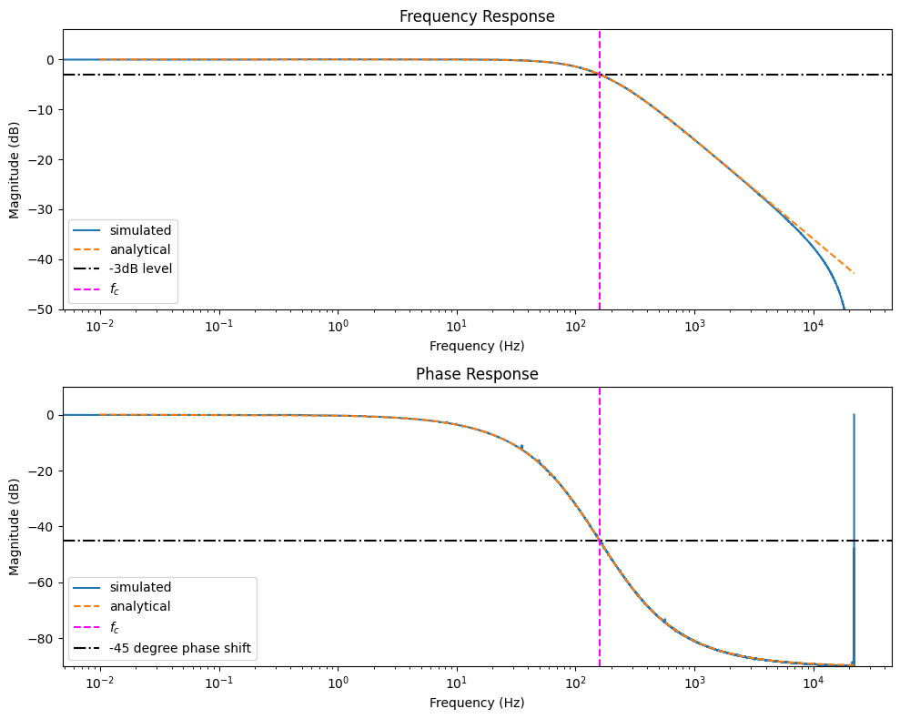
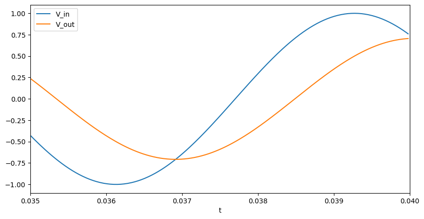
As we can see there is good agreement between the analytical prediction and the numerically measured response. The final plot shows that if we feed a sine wave in at
4 Passive RC Filter, 2nd order
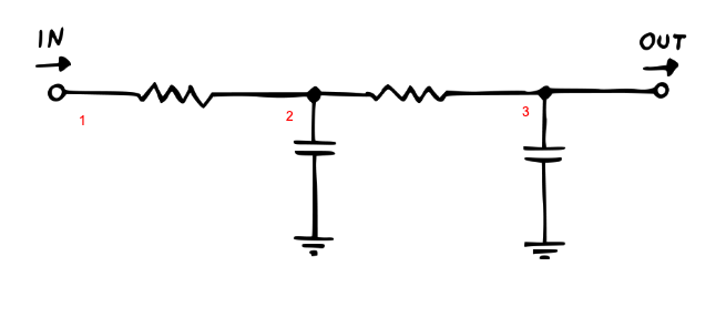
Let’s increase the complexity of the filter! We can stack multiple RC sections to apply a more aggressive filtering as shown above.
def solve_rc_filter_passive_2nd_order():
    netlist = """
    V0 1 0 Vin
    R 1 2 Rf
    C1 0 2 1.0e-6
    R 2 3 Rf
    C2 0 3 1.0e-6
    J 3 0
    """
    class_name = "RCFilter2ndOrder"
    rules, _ = run_MNA(netlist, class_name)

    code_string = generate_processor(rules)

    Rf, tmax, dt = 1000, 0.04, 1.0 / 44100.0
    ts = np.arange(0, tmax, dt)

    saw_fn = saw(freq=100, ppv=5.0)
    v_ins = saw_fn(ts)
    v_outs = []
    with ModuleLoader(code_string, class_name) as m:
        for v_in in v_ins:
            v_out = m.process(v_in, Rf, dt)
            v_outs.append(v_out)

    return ts, v_ins, v_outs


plt.figure(figsize=(10, 5))
plt.title(
    "Filtering a saw wave: comparison of 1st order and 2nd order passive RC filters"
)
plt.plot(ts, v_ins, label="V_in (100 Hz saw)")

ts, v_ins, v_outs_1eneg6 = solve_rc_filter_passive_1st_order(R=1000, C=1e-6, wave=saw)
plt.plot(
    ts, v_outs_1eneg6, label=f"V_out (f_c = {1/(2*np.pi*1000*1e-6):.4g} Hz) 1st Order"
)

ts, _, v_outs_rc_passive_2nd_order = solve_rc_filter_passive_2nd_order()
plt.plot(
    ts,
    v_outs_rc_passive_2nd_order,
    label=f"V_out (f_c = {1/(2*np.pi*1000*1e-6):.4g} Hz) 2nd Order",
)


plt.xlabel("time")
plt.legend()
plt.show()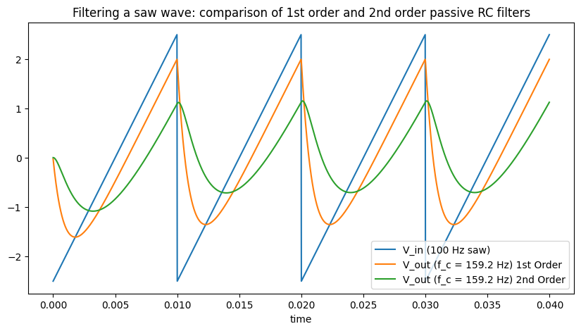
Comparing first and second order passive filters, we can see that the second order rounds off the saw even more strongly and the sharp discontinuity of the saw no longer remains. However as Moritz explains the second order passive isn’t truly a 2-pole filter, i.e., its filter response, or how much it attenuates a signal as a function of frequency, doesn’t match the expected characteristics (specifically the transition from the passband, where frequencies are allowed through, to the transition band, where there are increasingly attenuated, is too broad). This is better explained in the manual, but essentially the two stages interact with each other - this is solved by introducing an operational amplifier (op-amp) in the chain as a buffer.
5 Active RC Filter, 2nd order
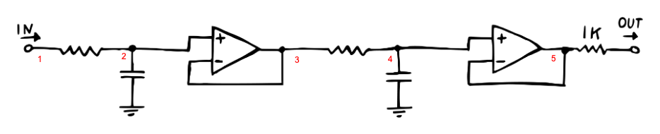
The active filter design places two op-amps, one after each 1st-order RC stage. In this case, we don’t actually require the second op-amp or output resistor - these are requirements only for the hardware version (e.g. to protect the buffer from short circuits.) This shows that in modeling circuits, we don’t always need to take a completely literal version of the circuit, and computational savings may be made removing such hardware protections.
def solve_rc_filter_active_2nd_order():
    # RC 2nd order active
    netlist = """
    V0 1 0 Vin
    R 1 2 Rf
    C1 2 0 1.0e-6
    OAmp 2 3 3
    R 3 4 Rf
    C2 4 0 1.0e-6
    J 4 0
    # OAmp 4 5 5   # we can skip the op-amp
    # R 5 6        # we can skip the output resistor
    """
    class_name = "RCFilter2ndOrderActive"
    rules, _ = run_MNA(netlist, class_name)

    code_string = generate_processor(rules)

    Rf, tmax, dt = 1000, 0.04, 1.0 / 44100.0
    ts = np.arange(0, tmax, dt)

    saw_fn = saw(freq=100, ppv=5.0)
    v_ins = saw_fn(ts)
    v_outs = []
    with ModuleLoader(code_string, class_name) as m:
        for v_in in v_ins:
            v_out = m.process(v_in, Rf, dt)
            v_outs.append(v_out)

    return ts, v_ins, v_outs


ts, _, v_outs_rc_active_2nd_order = solve_rc_filter_active_2nd_order()

plt.figure(figsize=(10, 5))
plt.title("Comparing passive vs active 2nd order RC filters")
plt.plot(ts, v_ins, label="V_in (100 Hz saw)")
plt.plot(
    ts,
    v_outs_rc_passive_2nd_order,
    label=f"V_out (f_c = {1/(2*np.pi*1000*1e-6):.4g} Hz) 2nd Order Passive",
)
plt.plot(
    ts,
    v_outs_rc_active_2nd_order,
    label=f"V_out (f_c = {1/(2*np.pi*1000*1e-6):.4g} Hz) 2nd Order Active",
)
plt.xlabel("time")
plt.legend()
plt.show()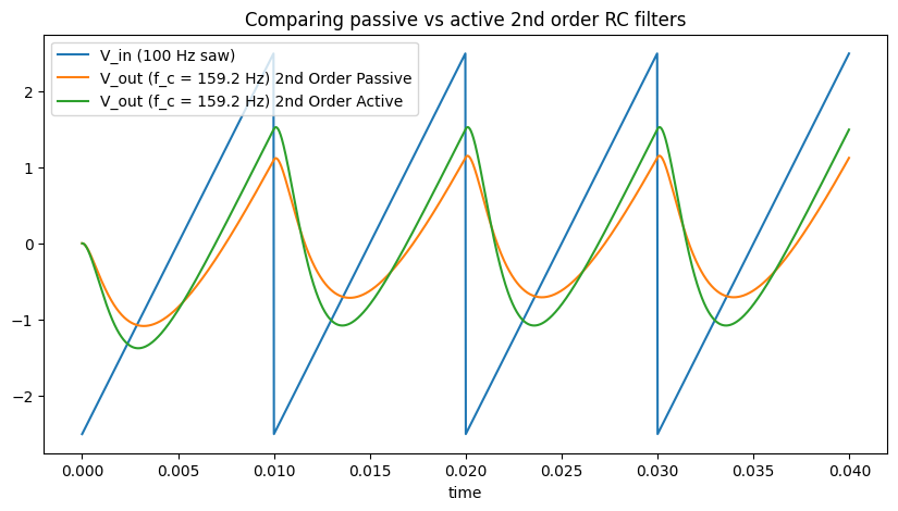
Comparing the passive and active filters, the main effect in the time domain is that we see less of an amplitude drop due to the buffer between the sections.
5.1 Frequency Response
We can again examine the frequency response of the passive and active filters. You can show that the expected cutoff frequency of first and second order RC filters goes as:
We can fit the 12 dB / octave slope and see where this intersects the 0dB line - this gives us a measurement for the cutoff frequency, which agrees well with the formula above (plotted in dashed magenta).
The cutoff frequency is typically defined as the frequency below which the power output has fallen by half (-3 dB). As we can see however, the -3dB line (dashed black) doesn’t intersect the curve at
We need to apply a correction
Finally we note that the passive 2nd order filter doesn’t meet the expected attenuation at
Code
def solve_rc_filter_active_2nd_order_response():
    Rf = 1000
    C = 1e-6
    order = 2  # second order

    # RC 2nd order active
    netlist = f"""
    V0 1 0 Vin
    R 1 2 Rf
    C1 2 0 {C}
    OAmp 2 3 3
    R 3 4 Rf
    C2 4 0 {C}
    J 4 0
    # OAmp 4 5 5   # we can skip the op-amp
    # R 5 6        # we can skip the output resistor
    """
    class_name_active = "RCFilter2ndOrderActiveResponse"
    rules, _ = run_MNA(netlist, class_name_active)
    code_string_active = generate_processor(rules)

    netlist = f"""
    V0 1 0 Vin
    R 1 2 Rf
    C1 0 2 {C}
    R 2 3 Rf
    C2 0 3 {C}
    J 3 0
    """
    class_name_passive = "RCFilter2ndOrderPassiveResponse"
    rules, _ = run_MNA(netlist, class_name_passive)
    code_string_passive = generate_processor(rules)

    with ModuleLoader(code_string_active, class_name_active) as m_active, ModuleLoader(
        code_string_passive, class_name_passive
    ) as m_passive:
        fig, ax = plt.subplots(figsize=(12, 6))
        plot_filter_response(m_active, ax=ax, args=(Rf,), label="active")
        plot_filter_response(m_passive, ax=ax, args=(Rf,), label="passive")

        # plot the -3dB line
        ax.axhline(-3, linestyle="-.", color="black", label="-3dB level")
        # and where we expect the cutoff to be
        cutoff_expected = 1 / (2 * np.pi * Rf * C)
        ax.axvline(cutoff_expected, linestyle="--", color="magenta", label="$f_c$")
        # where it actually is (red)!
        cutoff_actual = cutoff_expected * np.sqrt(np.power(2, 1 / order) - 1)
        ax.axvline(
            cutoff_actual,
            linestyle="--",
            color="cyan",
            label="$f_{-3dB} = f_c \sqrt{2^{1/2} - 1}$",
        )

        # plot a trendline just for reference, where we expect 12dB / oct for 2nd order
        octaves = 6.5
        ax.plot(
            [9e3, 9e3 / (2**octaves)],
            [-70, -70 + (octaves * 12)],
            "--",
            color="#1f77b4",
            label="12dB / oct",
        )
        ax.axhline(0, linestyle="--", color="#1f77b4")

        passive_filter_gain_at_fc = 20 * np.log10((1 / np.sqrt(2)) ** order)
        ax.axhline(
            passive_filter_gain_at_fc,
            linestyle="-.",
            color="#ff7f0e",
            label="passive 2nd order gain at $f_{-3dB}$",
        )

        ax.plot(cutoff_actual, -3, "o", color="#1f77b4")
        ax.plot(cutoff_actual, passive_filter_gain_at_fc, "o", color="#ff7f0e")

        ax.legend()
        ax.grid()
        plt.show()


solve_rc_filter_active_2nd_order_response()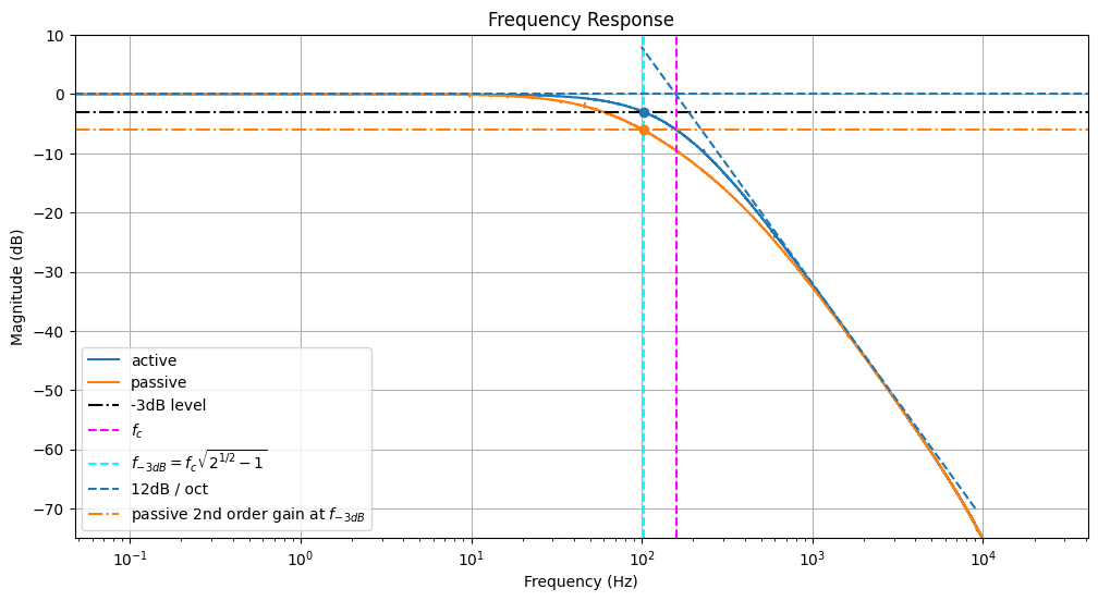
6 Nth Order RC Filters
6.1 Active Filters
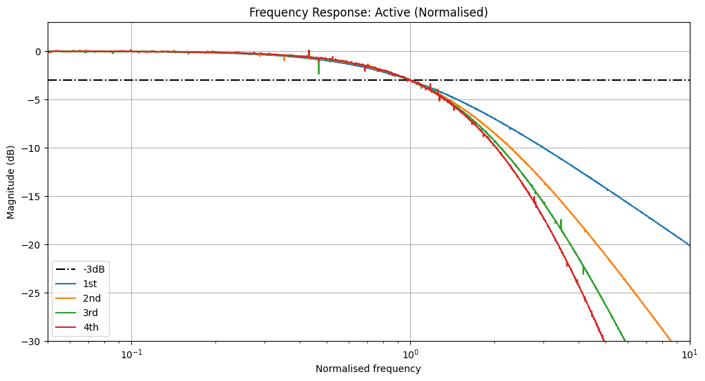
Because we can solve this programmatically, we can easily extend to arbitrary higher orders with a for loop for fun! Below are shown the responses for 1st, 2nd, 3rd, and 4th order active RC filters. Note how both the predicted and measured -3dB attentuation frequency shifts left with higher order filters.
Plotted are the expected attenuation slopes (dashed lines, slope of order
Code
def solve_rc_filter_active_nth_order_response(normalise_frequencies: bool):
    Rf = 1000

    fig, ax = plt.subplots(figsize=(12, 6))

    # plot the -3dB line
    ax.axhline(-3, linestyle="-.", color="black", label="-3dB")
    # and where we expect the cutoff to be
    cutoff_expected = 1 / (2 * np.pi * Rf * 1e-6)

    labels = ["1st", "2nd", "3rd", "4th"]

    netlist = "V0 1 0 Vin"
    for n in range(0, 4):
        order = n + 1

        # append the netlist to add successive (buffered) RC sections
        netlist += f"""
R {1 + 2*n} {2 + 2*n} Rf
C{n} {2 + 2*n} 0 1.0e-6
OAmp {2 + 2*n} {3 + 2*n} {3 + 2*n}"""

        # where it actually is (red)!
        cutoff_actual = cutoff_expected * np.sqrt(np.power(2, 1 / order) - 1)
        ax.axvline(cutoff_actual, linestyle="-.", color=colors[n])

        class_name = f"RCFilterResponse_{order}thActive"
        output_node_str = f"\nJ {3 + 2*n} 0"
        rules, _ = run_MNA(netlist + output_node_str, class_name)
        code_string = generate_processor(rules)

        with ModuleLoader(code_string, class_name) as m:
            frequency_scale = cutoff_actual if normalise_frequencies else 1.0
            title = "Frequency Response: Active"
            if normalise_frequencies:
                title += " (Normalised)"

            plot_filter_response(
                m,
                ax=ax,
                args=(Rf,),
                label=labels[n],
                title=title,
                frequency_scale=frequency_scale,
            )

        # plot a trendline just for reference, where we expect order*6dB / oct for nth order
        octaves = 5
        if not normalise_frequencies:
            ax.plot(
                [cutoff_expected, cutoff_expected * (2**octaves)],
                [0, -(octaves * 6 * order)],
                "--",
                color=colors[n],
            )

        ax.plot(cutoff_actual, -3, "o", color=colors[n])

    ax.scatter(cutoff_expected, 0, marker="*", color="k", s=100)

    if normalise_frequencies:
        ax.set_xlim(0.05, 10)
        ax.set_ylim(-30, 3)

        ax.set_xlabel("Normalised frequency")
    else:
        ax.set_xlim(5, 1e4)
        ax.set_ylim(-60, 6)
    ax.legend()
    ax.grid()
    plt.show()


solve_rc_filter_active_nth_order_response(False)
solve_rc_filter_active_nth_order_response(True)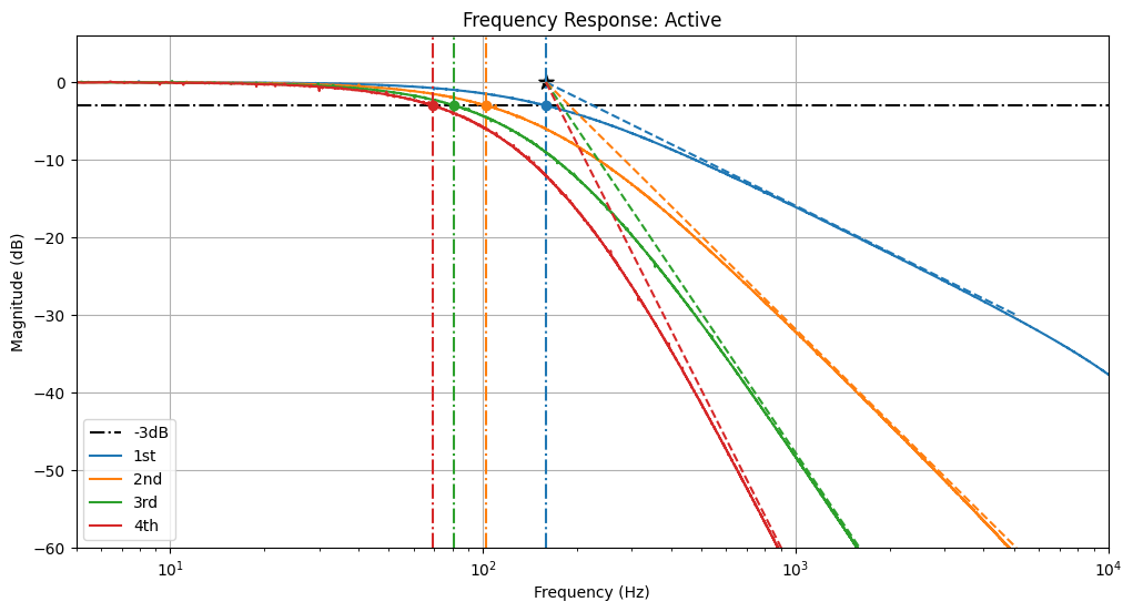
6.2 Passive Filters
We can repeat the experiment with passive RC filters. Note how the attenuation slopes converge at a constant
Plotted are the expected attenuation slopes (dashed lines, slope of order
Code
def solve_rc_filter_passive_nth_order_response():
    Rf = 1000

    fig, ax = plt.subplots(figsize=(12, 6))

    # and where we expect the cutoff to be
    cutoff_expected = 1 / (2 * np.pi * Rf * 1e-6)

    labels = ["1st", "2nd", "3rd", "4th"]

    netlist = "V0 1 0 Vin"
    for n in range(0, 4):
        order = n + 1

        # append the netlist to add successive RC sections
        netlist += f"""
R {1 + n} {2 + n} Rf
C{n+1} {2 + n} 0 1.0e-6"""

        # where it actually is (red)!
        cutoff_actual = cutoff_expected * np.sqrt(np.power(2, 1 / order) - 1)
        ax.axvline(cutoff_actual, linestyle="-.", color=colors[n])

        class_name = f"RCFilterResponse_{order}thPassive"
        output_node_str = f"\nJ {2 + n} 0"
        rules, _ = run_MNA(netlist + output_node_str, class_name)
        code_string = generate_processor(rules)

        with ModuleLoader(code_string, class_name) as m:
            plot_filter_response(
                m,
                ax=ax,
                args=(Rf,),
                label=labels[n],
                title="Frequency Response: Passive",
            )

        # plot a trendline just for reference, where we expect order*6dB / oct for nth order
        octaves = 5
        ax.plot(
            [cutoff_expected, cutoff_expected * (2**octaves)],
            [0, -(octaves * 6 * order)],
            "--",
            color=colors[n],
        )

        passive_filter_gain_at_fc = 20 * np.log10((1 / np.sqrt(2)) ** order)
        ax.plot(cutoff_actual, passive_filter_gain_at_fc, "o", color=colors[n])
        ax.axhline(passive_filter_gain_at_fc, linestyle="-.", color=colors[n])

    orders = np.linspace(0.5, 9)
    xs = cutoff_expected * np.sqrt(np.power(2, 1 / orders) - 1)
    ys = 20 * np.log10(np.power(1 / np.sqrt(2), orders))
    ax.plot(xs, ys, "-.", color="k")

    ax.scatter(cutoff_expected, 0, marker="*", color="k", s=100)

    ax.set_xlim(5, 1e4)
    ax.set_ylim(-70, 6)
    ax.legend()
    plt.show()


solve_rc_filter_passive_nth_order_response()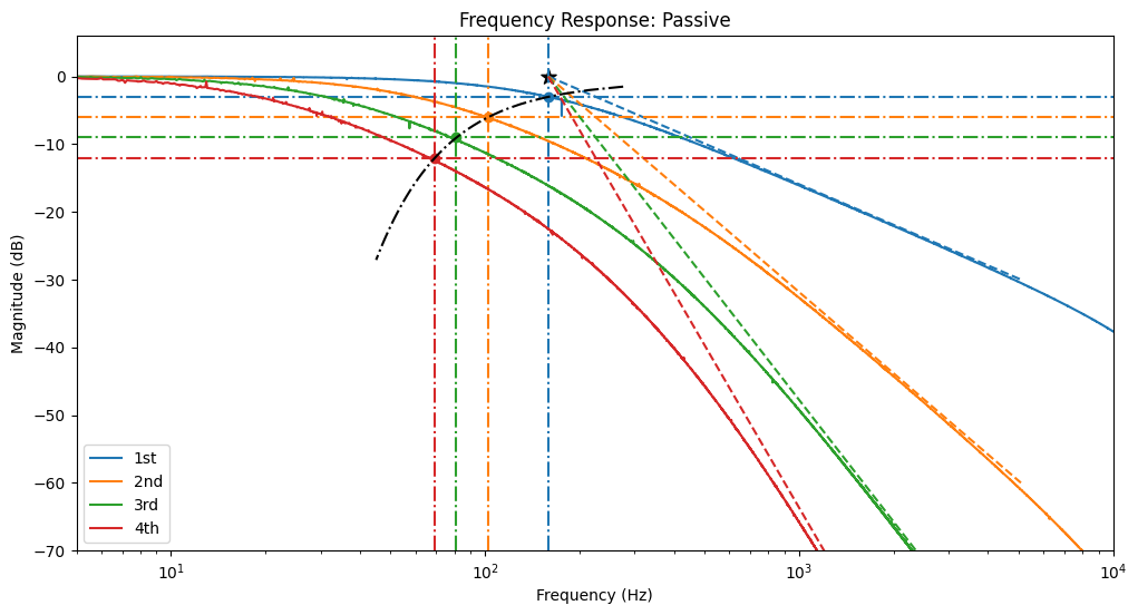
7 Comparison to hardware
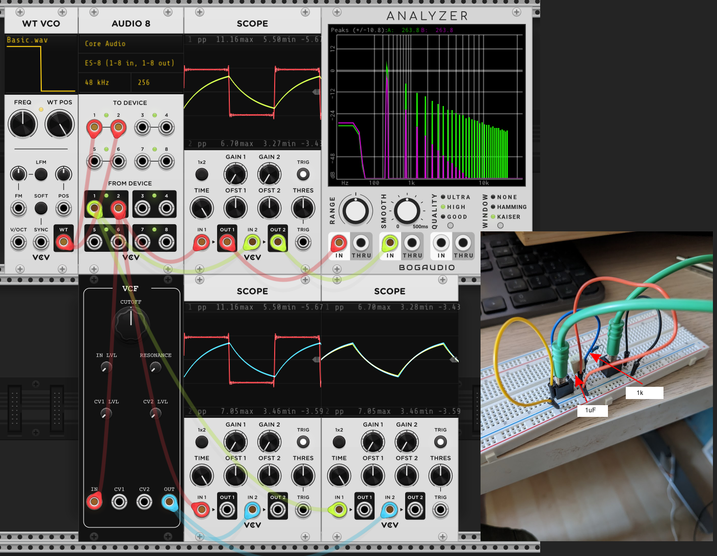
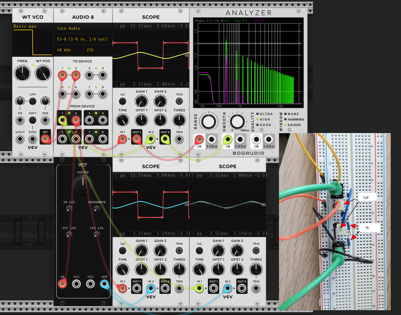
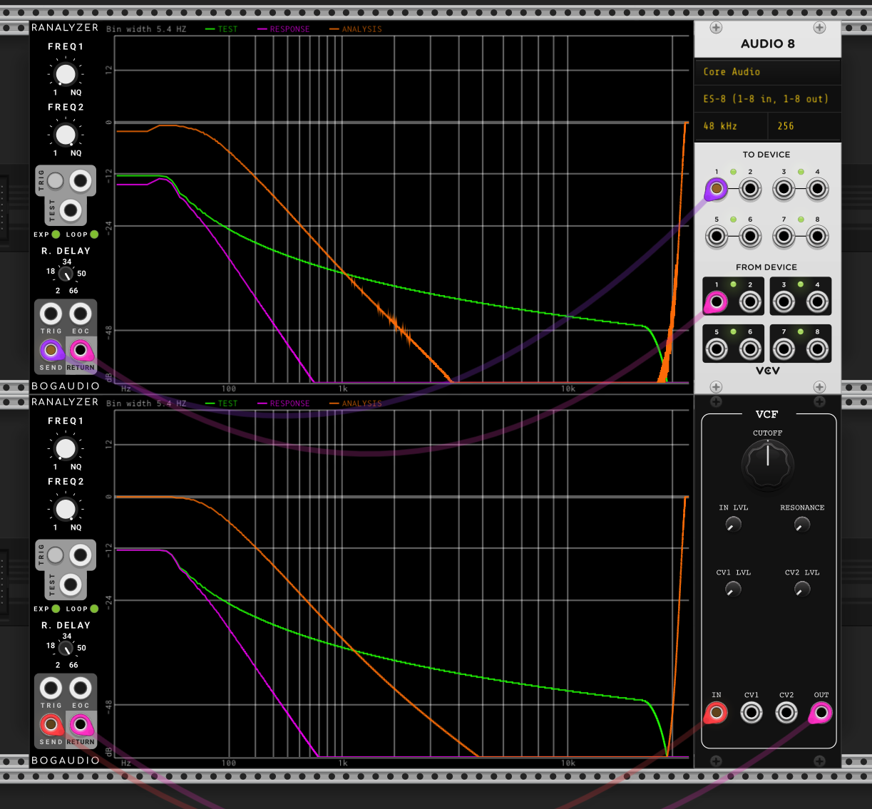
Everything shown so far is completely theoretical or simulated. The final proof is whether these simulations match the circuits. I’ve breadboarded these up (see inset photos) and send signals from VCV Rack, through the breadboard then back in again using the Expert Sleepers ES-8 interface.
7.1 Passive RC Filter, 1st order
7.2 Passive RC Filter, 2nd order
8 Conclusions
By combining very simple elements, resistors, capacitors and sometimes (ideal) op-amps, we can simulate and recreate members of one of the simplest families of filter - the RC filter. In the Part 2, we look at adding resonance to these designs.