Reproducing Andrew Simper ADC 2020

1 Intro

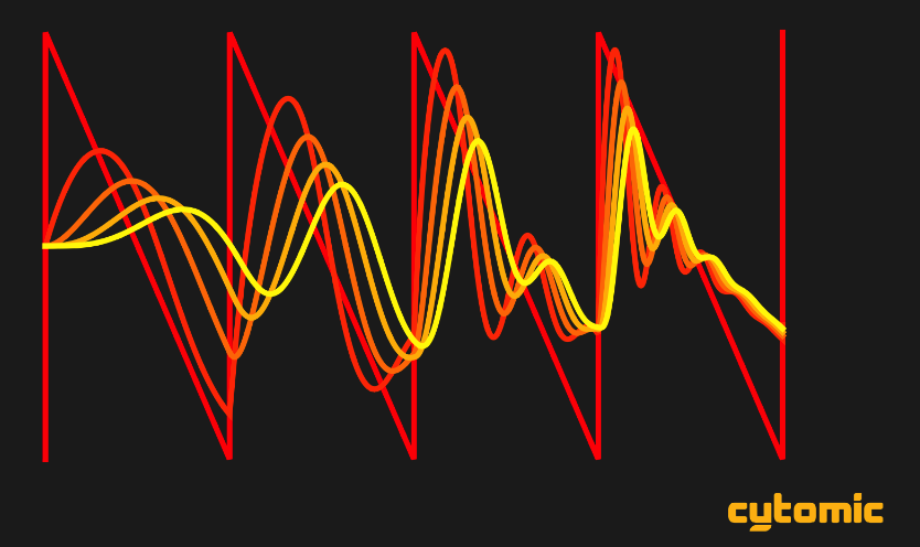
Screengrab from ADC 2020 slides

Andrew Simper gave a great talk at ADC 2020 conference (slides here) covering a wide range of topics in circuit modeling. This was one of the first times I was exposed to the details of circuit modeling and it really sparked my interest. Here we’ll investigate some of the simple circuits presented there.

2 LPF, HPF

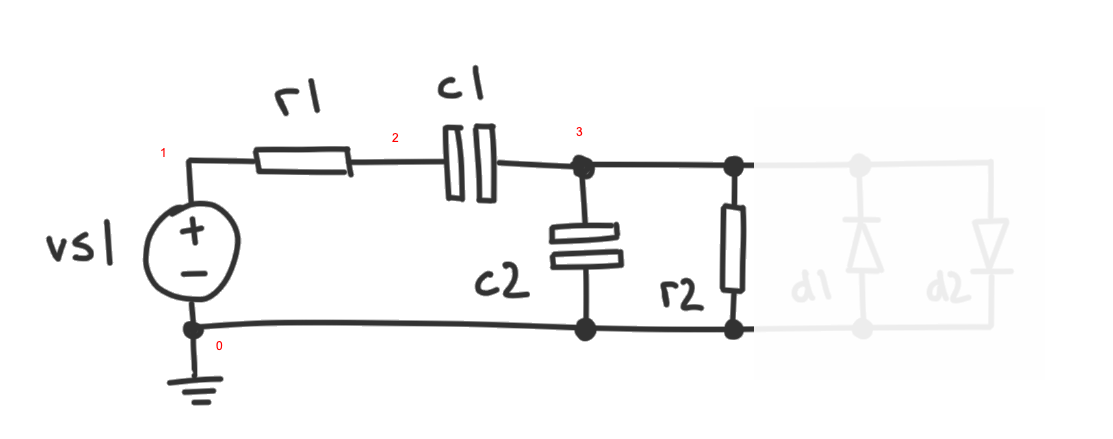
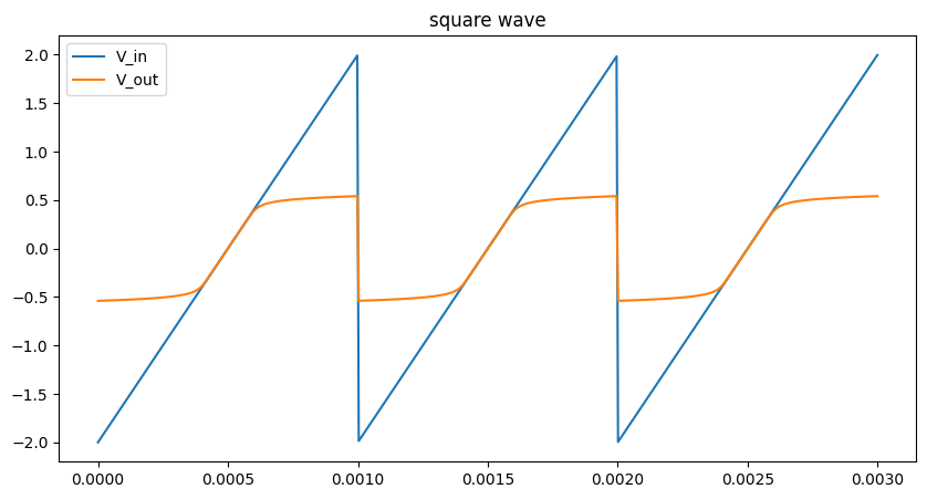
Figure 1: 1 pole lowpass, 1 pole highpass

We start with the 1 pole lowpass, 1 pole highpass filter. If you’ve not already, it is worth looking at the previous post VCF: Part 1 - RC Filters.

A little work is needed to use the notation in Andrew’s slides, we use the assumptions argument to map between the naming schemes.

Code

def generate_lpfhpf_maths():
    # chained lpf, hpf
    netlist = """
    V0 1 0 V_in
    R1 1 2 R1
    C1 3 2 0.47e-6
    C2 3 0 0.01e-6
    R2 3 0 R2
    J 3 0
    """
    
    # switch to symbols used in notes briefly
    R1, gr1, R2, gr2 = symbols('R1, gr1, R2, gr2')
    c1gc, gc1, c2gc, gc2 = symbols('c1.gc, gc1, c2.gc, gc2')
    c1ieq, ic1eq, c2ieq, ic2eq = symbols('c1.ieq, ic1eq, c2.ieq, ic2eq')
    assumptions = {R1: 1/gr1, R2: 1/gr2, c1gc: gc1, c2gc: gc2, c1ieq: ic1eq, c2ieq: ic2eq}    
    class_name = "RCBand"  + str(np.random.randint(100000))        
    rules, (A, x, b) = run_MNA(netlist, class_name, assumptions=assumptions, method="LUsolve")
    
    display(Markdown("## Solutions from SPICEWORLD code"))
    display(Markdown("The auto-generated matrix problem reads:"))
    
    display(Eq(MatMul(A, x), b))
    display(Eq(Mul(A, x), b))
    
    display(Markdown("Pulling out the second and third rows reads:"))
    kcl = (A*x-b)
    display(Eq(0, kcl[1]))
    display(Eq(0, kcl[2]))
    
    v_2, v_3, V_in = symbols("v_2, v_3, V_in")
    
    v_3_spiceworld = rules.solutions[3].rhs
    v_2_spiceworld = rules.solutions[2].rhs
    
    # little manipulation to get into same format
    v_3_num, v_3_denom = fraction(factor(v_3_spiceworld))
    v_3_v_3_denomnum = collect(v_3_denom, [gr1, gc1])
    v_3_num = collect(v_3_num, [gr1])
    v_3_spiceworld = v_3_num / v_3_denom
    display(Markdown("This yields solutions from SPICEWORLD, which after a little re-ordering reads:"))
    display(Eq(v_3, v_3_spiceworld))
    display(Eq(v_2, v_2_spiceworld))
    
    display(Markdown("## Solutions from talk"))
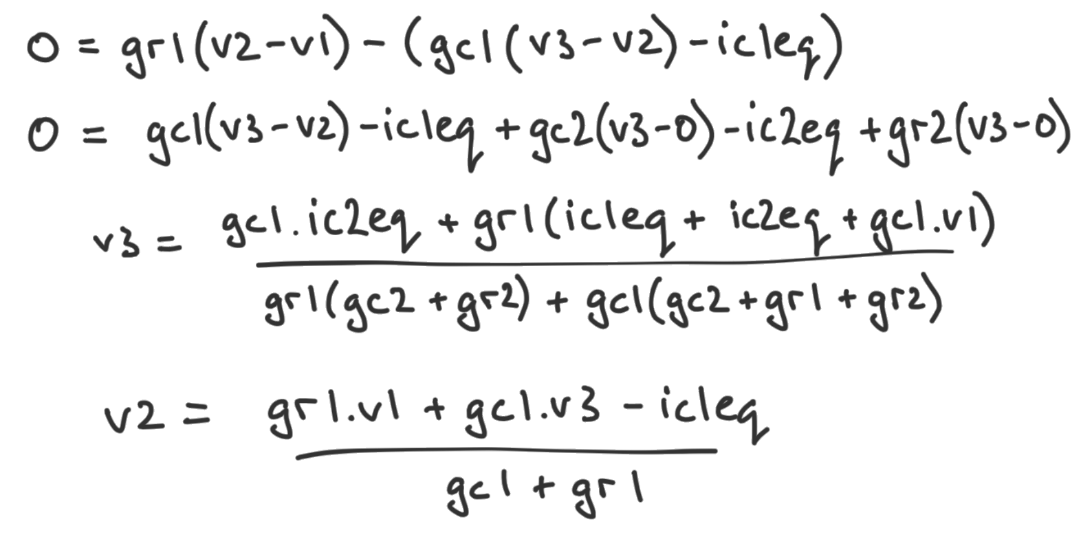
    display(Markdown("![Equations for LPF, HPF voltages](./eqns.png){width=500}"))
    display(Markdown("Writing these out in sympy form, we can verify that they are the same"))
    
    v_3_simper = (gc1 * ic2eq + gr1*(ic1eq + ic2eq + gc1*V_in)) / (gr1*(gc2 + gr2) + gc1*(gc2 + gr1 + gr2))        
    v_2_simper = (gr1*V_in + gc1*v_3 - ic1eq) / (gc1 + gr1)
    display(Eq(v_3, v_3_simper))
    display(Eq(v_2, v_2_simper))
    
    display(Markdown("If we substitude v_3 in, we get the final expression for v_2 that matches the SPICEWORLD solution. "))
    v_2_simper = simplify(v_2_simper.subs({v_3: v_3_simper}))
    display(Eq(v_2, v_2_simper))
    
    # prove solutions are the same
    assert simplify(v_3_spiceworld-v_3_simper) == 0
    assert simplify(v_2_spiceworld-v_2_simper) == 0
    
generate_lpfhpf_maths()

2.1 Solutions from SPICEWORLD code

The auto-generated matrix problem reads:

${\displaystyle \left[\begin{array}{cccc}g{r}_1& -g{r}_1& 0& 1\\ -g{r}_1& g{c}_1+g{r}_1& -g{c}_1& 0\\ 0& -g{c}_1& g{c}_1+g{c}_2+g{r}_2& 0\\ 1& 0& 0& 0\end{array}\right]\left[\begin{array}{c}{v}_1\\ v_2\\ v_3\\ i_{v1}\end{array}\right]=\left[\begin{array}{c}0\\ -ic1eq\\ ic1eq+ic2eq\\ V_{in}\end{array}\right]}$

${\displaystyle \left[\begin{array}{c}g{r}_1{v}_1-g{r}_1{v}_2+i_{v1}\\ -g{c}_1{v}_3-g{r}_1{v}_1+v_2(g{c}_1+g{r}_1)\\ -g{c}_1{v}_2+v_3(g{c}_1+g{c}_2+g{r}_2)\\ v_1\end{array}\right]=\left[\begin{array}{c}0\\ -ic1eq\\ ic1eq+ic2eq\\ V_{in}\end{array}\right]}$

Pulling out the second and third rows reads:

${\displaystyle 0=-g{c}_1{v}_3-g{r}_1{v}_1+ic1eq+v_2(g{c}_1+g{r}_1)}$

${\displaystyle 0=-g{c}_1{v}_2-ic1eq-ic2eq+v_3(g{c}_1+g{c}_2+g{r}_2)}$

This yields solutions from SPICEWORLD, which after a little re-ordering reads:

${\displaystyle v_3=\frac{g{c}_{1}ic2eq+g{r}_1(V_{in}g{c}_1+ic1eq+ic2eq)}{g{c}_{1}g{c}_2+g{c}_{1}g{r}_1+g{c}_{1}g{r}_2+g{c}_{2}g{r}_1+g{r}_{1}g{r}_2}}$

${\displaystyle v_2=\frac{V_{in}g{c}_{1}g{r}_1+V_{in}g{c}_{2}g{r}_1+V_{in}g{r}_{1}g{r}_2+g{c}_{1}ic2eq-g{c}_{2}ic1eq-g{r}_{2}ic1eq}{g{c}_{1}g{c}_2+g{c}_{1}g{r}_1+g{c}_{1}g{r}_2+g{c}_{2}g{r}_1+g{r}_{1}g{r}_2}}$

2.2 Solutions from talk

Equations for LPF, HPF voltages

Writing these out in sympy form, we can verify that they are the same

${\displaystyle v_3=\frac{g{c}_{1}ic2eq+g{r}_1(V_{in}g{c}_1+ic1eq+ic2eq)}{g{c}_1(g{c}_2+g{r}_1+g{r}_2)+g{r}_1(g{c}_2+g{r}_2)}}$

${\displaystyle v_2=\frac{V_{in}g{r}_1+g{c}_1{v}_3-ic1eq}{g{c}_1+g{r}_1}}$

If we substitude v_3 in, we get the final expression for v_2 that matches the SPICEWORLD solution.

${\displaystyle v_2=\frac{V_{in}g{c}_{1}g{r}_1+V_{in}g{c}_{2}g{r}_1+V_{in}g{r}_{1}g{r}_2+g{c}_{1}ic2eq-g{c}_{2}ic1eq-g{r}_{2}ic1eq}{g{c}_{1}g{c}_2+g{c}_{1}g{r}_1+g{c}_{1}g{r}_2+g{c}_{2}g{r}_1+g{r}_{1}g{r}_2}}$

Let’s numerically solve this system of equations.

def generate_lpfhpf(ts ,v_ins):
    # chained lpf, hpf
    netlist = """
    V0 1 0 Vin
    R1 1 2 R1
    C1 2 3 0.47e-6
    C2 3 0 0.01e-6
    R2 3 0 R2    
    J 3 0
    """
    
    class_name = "RCBand"  + str(np.random.randint(100000))        
    rules, (A, x, b) = run_MNA(netlist, class_name, assumptions={}, method="LUsolve")
    code_string = generate_processor(rules)

    fig, axs = plt.subplots(2, 1, figsize=(10, 8))
            
    with ModuleLoader(code_string, class_name) as m:       
                
        R1, R2 = 2230, 6800
        
        v_outs = []    
        for v_in in v_ins:
            v_outs.append(m.process(v_in, R1, R2, dt))            

        v_outs = np.array(v_outs)
        axs[0].set_title('square wave')
        axs[0].plot(ts, v_ins, label='V_in')
        axs[0].plot(ts, v_outs, label='V_out')
        axs[0].legend()
            
        for i, Rf in enumerate([0.1, 1, 10]):
            R1, R2 = Rf * 2230, Rf*6800
            plot_filter_response(m, ax=axs[1], args=(R1, R2), title='Frequency Response: Resonance', 
                                 label=f'$Rf = {Rf} * R_1, R_2$', sampling_frequency=88200.)
        
            # where we expect the cutoff to be            
            cutoff_expected = 1/(2*np.pi*Rf*1e-6)
            axs[1].axvline(cutoff_expected, linestyle=':', color=colors[i])
    
    axs[1].set_xlim(0.3, 1e5)
    axs[1].set_ylim(-30, 6)
    plt.show()
    
    return v_outs
    
# x4 oversampled at 44100. (effectively)
tmax, dt = 0.003, 0.25/44100.
ts = np.arange(0, tmax, dt)        
fn = saw(freq=1000, ppv=4.)    
v_ins = fn(ts)

v_outs_lpfhpf = generate_lpfhpf(ts, v_ins)

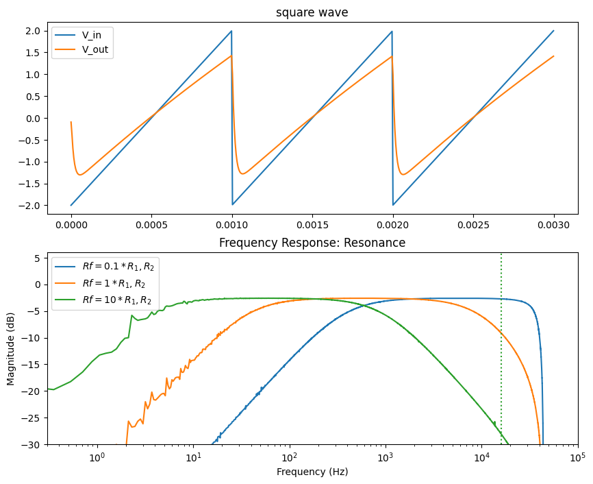
We can see a nice bandpass frequency response, and the waveform broadly matches that displayed in the slides.

3 Diode

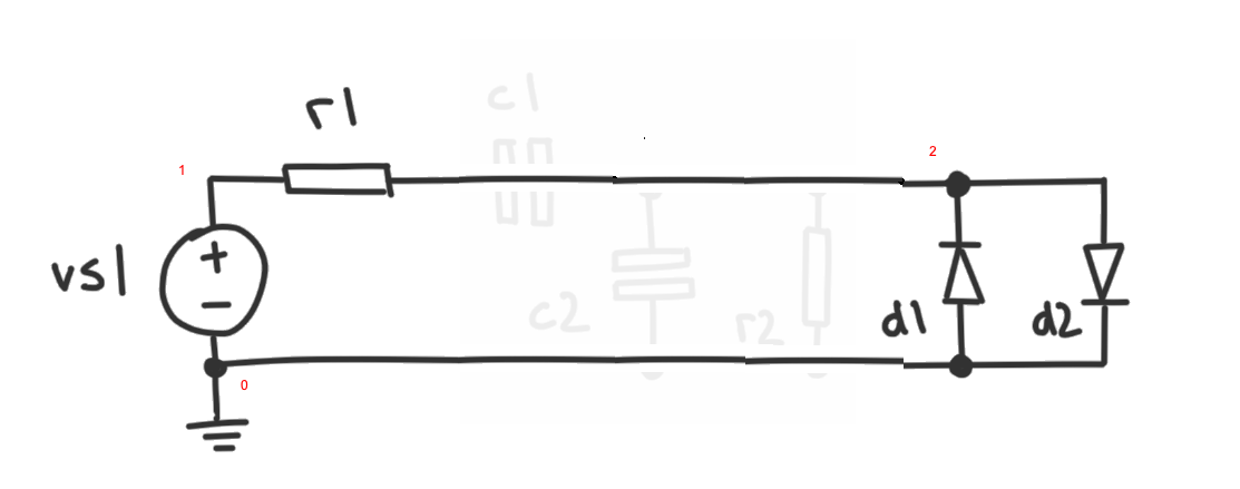
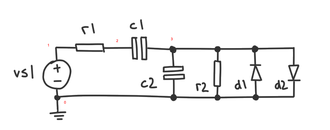
Figure 2: Diode Clipper

We’ll cover diode clipping elsewhere in more detail, so for now we just reproduce the clipper using the netlist derived from the above simple circuit. As we can see, there is a nice saturation applied to the saw.

def generate_diode_clipper(ts, v_ins, plot=True):
    netlist = """
    V0 1 0 Vin
    R1 1 2 2200    
    D1 0 2 
    D2 2 0 
    J 2 0
    """
    class_name = "DiodeClipper"  + str(np.random.randint(100000))  
    rules, (A, x, b) = run_MNA(netlist, class_name)
    code_string = generate_processor(rules)
        
    with ModuleLoader(code_string, class_name) as m:       

        v_outs = []    
        for v_in in v_ins:
            v_outs.append(m.process(v_in, dt))            

        v_outs = np.array(v_outs)
        
        if plot:
            fig, axs = plt.subplots(1, 1, figsize=(10, 5))
            axs.set_title('square wave')
            axs.plot(ts, v_ins, label='V_in')
            axs.plot(ts, v_outs, label='V_out')
            axs.legend()
            plt.show()
            
    return v_outs

v_outs_diode_clipper = generate_diode_clipper(ts, v_ins)

4 Filter (Full)

Figure 3: Full filter

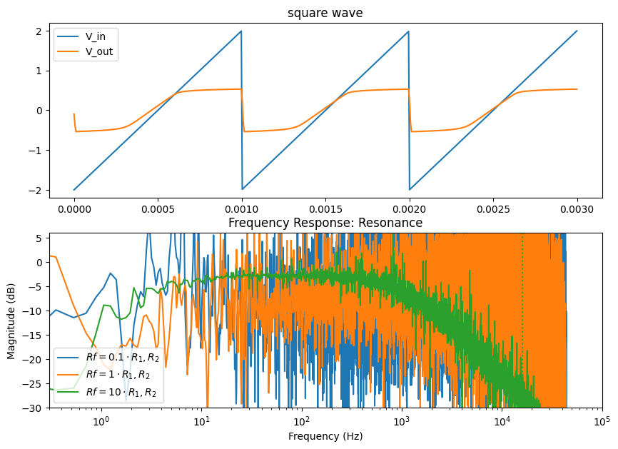
Finally we can put together the full filter, including diodes. Note that now the filter is nonlinear, the frequency response is no longer defined, and indeed we get an uninterpretable mess from it!

def generate_full(ts, v_ins):
    # chained lpf, hpf and diodes
    netlist = """
    V0 1 0 Vin
    R1 1 2 R1
    C1 2 3 0.47e-6
    C2 3 0 0.01e-6
    R2 3 0 R2   
    D1 3 0
    D2 0 3
    J 3 0
    """
    
    class_name = "RCBand"  + str(np.random.randint(100000))        
    rules, (A, x, b) = run_MNA(netlist, class_name, assumptions={}, method="LUsolve")
    code_string = generate_processor(rules)

    fig, axs = plt.subplots(2, 1, figsize=(10, 7))
            
    with ModuleLoader(code_string, class_name) as m:       

        R1, R2 = 2230, 6800
        
        v_ins = fn(ts)
        v_outs = []    
        for v_in in v_ins:
            v_outs.append(m.process(v_in, R1, R2, dt))            

        v_outs = np.array(v_outs)
        axs[0].set_title('square wave')
        axs[0].plot(ts, v_ins, label='V_in')
        axs[0].plot(ts, v_outs, label='V_out')
        axs[0].legend()
            
        for i, Rf in enumerate([0.1, 1, 10]):
            R1, R2 = Rf * 2230, Rf*6800
            plot_filter_response(m, ax=axs[1], args=(R1, R2), title='Frequency Response: Resonance', 
                                 label=f'$Rf = {Rf} \cdot R_1, R_2$', sampling_frequency=88200.)
        
            # where we expect the cutoff to be            
            cutoff_expected = 1/(2*np.pi*Rf*1e-6)
            axs[1].axvline(cutoff_expected, linestyle=':', color=colors[i])
    
    axs[1].set_xlim(0.3, 1e5)
    axs[1].set_ylim(-30, 6)
    plt.show()
    
    return v_outs

v_outs_full = generate_full(ts, v_ins)

We can also compare the full model with the serial (LPF/HPF into clipper), and indeed we can see some subtle differences to the waveform.

v_outs_lpfhpf_then_diode = generate_diode_clipper(ts, v_outs_lpfhpf, plot=False)

fig, axs = plt.subplots(2, 1, figsize=(10, 10))
for i, ax in enumerate(axs):
    if i == 0:
        ax.plot(ts, v_outs_lpfhpf, label='LPF, HPF')
        
    ax.plot(ts, v_outs_lpfhpf_then_diode, label='hp lp -> clip')
    ax.plot(ts, v_outs_full, label='full model')
    ax.legend()
    ax.grid()
    
axs[1].set_ylim(-0.6, +0.6)
plt.show()

5 Frequency Response and Integration Method

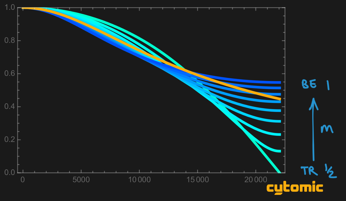
Figure 4: Effect of numerical method on frequency response

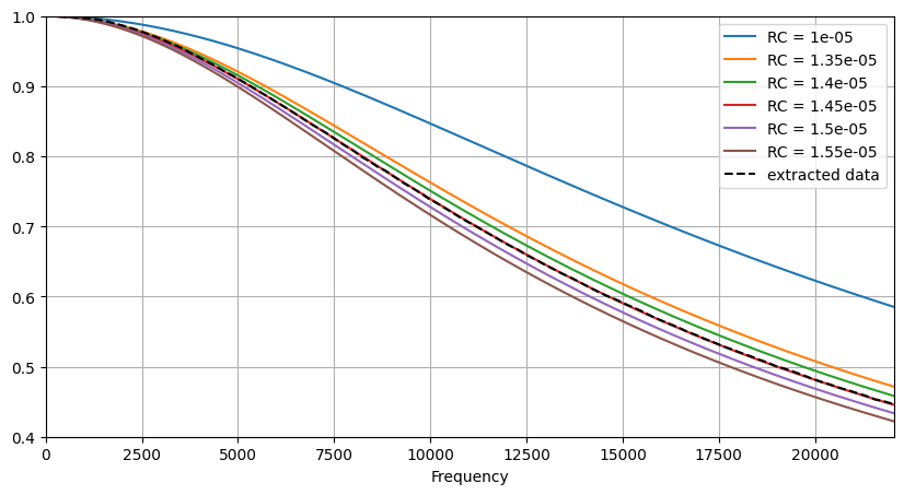
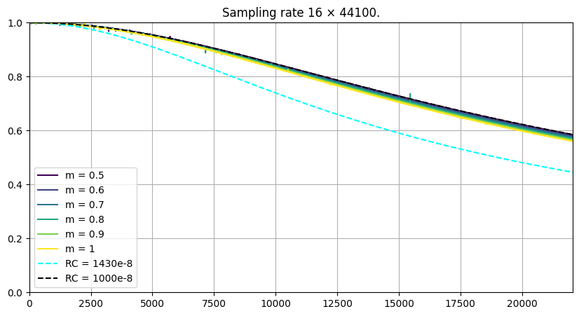
Lastly the talk describes the effect of integration method on the frequency response, with the example given as an RC filter. First lets extract the ideal curve data (yellow curve) to work out what $R\times C$ is - from below, we see $RC\approx 1450\times {10}^{-8}$. This is perhaps a mistake in the data generation process, as we’ll try and show below.

fig, ax = plt.subplots(figsize=(10, 5))
f = np.linspace(0.01, 22050, 200)

for RC in [1000e-8, 1350e-8, 1400e-8, 1450e-8, 1500e-8, 1550e-8]:
    fc = 1.0/(2*np.pi*RC)

    gain = (fc / f) / np.sqrt(1 + np.power(fc / f, 2))  
    ax.plot(f, gain, label=f'RC = {RC:.4g}')

a = np.loadtxt("extracted.csv")
ax.plot(a[:, 0], a[:, 1], "--", color='k', label='extracted data')
    
ax.grid()
ax.set_ylim(0.4, 1)
ax.set_xlim(0, 22050)
ax.set_xlabel('Frequency')
ax.legend()
plt.show()

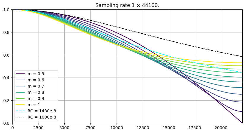
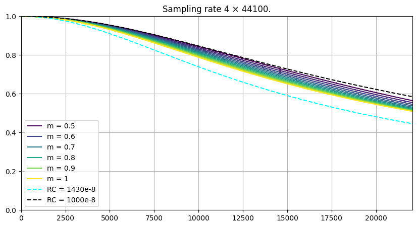
Next let’s solve the numerical problem as a function of numerical method $m$, where $m=0.5$ is trapezoidal method and $m=1$ is backward Euler. If instead we use $R\times C=1000\times {10}^{-8}$, we can reproduce the numerical results. Additionally increasing the sampling rate (or decreasing the timestep) we eventually recover the theoretical limit corresponding to $RC=1000\times {10}^{-8}$, suggesting that the yellow curve plotted in Figure 4 the slides is not correct.

def integration_method_response(a):
    def integration_method_response_inner(options, a):
        netlist = f"""
        V0 1 0 Vin
        R1 1 2 1000
        C1 2 0 1e-8 {options}
        J 2 0
    """
        class_name = "CapTest"  + str(np.random.randint(100000))  
        rules, _ = run_MNA(netlist, class_name)
        code_string = generate_processor(rules)

        with ModuleLoader(code_string, class_name) as m:

            f, H_dB, H, phi_deg = calculate_filter_response(m, sampling_frequency=a*44100)

        return f, H_dB, H, phi_deg

    fig, ax =  plt.subplots(figsize=(10, 5))
    for i, m in enumerate([0.5, 0.55, 0.6, 0.65, 0.7, 0.75, 0.8, 0.85, 0.9, 0.95, 1]):
        f, H_dB, H, phi_deg = integration_method_response_inner(f'm={m}', a)
        label = "" if i % 2 else f"m = {m}"
        ax.plot(f, H, color=viridis_11.colors[i], label=label)
    ax.set_xscale('linear')
    ax.set_yscale('linear')
    ax.set_xlim(0, 44100. / 2)
    ax.set_ylim(0.0, 1)
    ax.set_title(f"Sampling rate {a} × 44100.")
    
    # drop the zero entry (divide by zero below!)
    f = f[1:]
    
    RC = 1450e-8    
    fc = 1.0/(2*np.pi*RC)
    gain = (fc / f) / np.sqrt(1 + np.power(fc / f, 2))
    ax.plot(f, gain, "--", color='cyan', label='RC = 1430e-8')
    
    RC = 1000e-8
    fc = 1.0/(2*np.pi*RC)
    gain = (fc / f) / np.sqrt(1 + np.power(fc / f, 2))
    ax.plot(f, gain, "--", color='k', label='RC = 1000e-8')
    ax.grid()
    
    ax.legend()
    plt.show()
    
integration_method_response(1)
integration_method_response(4)
integration_method_response(16)