netlist = """
Vi 1 0 Vin
C1 1 2 0.25e-9
Pt 3 7 2 250.0e3
R2 3 4 R2
Pm 0 5 4 25.0e3
C3 5 6 20e-9
C2 3 6 20e-9
R4 1 6 56.0e3
J 7 0
"""
class_name = "ToneStack"
R2, yl = symbols("R2 yl")
rules, (A, x, b) = run_MNA(
    netlist, class_name, assumptions={R2: yl * R2}, method="LUsolve", simplify_sol=False
)
rules.constants.append(Assignment(R2, 1.0e6))

code_string = generate_processor(rules)1 Intro
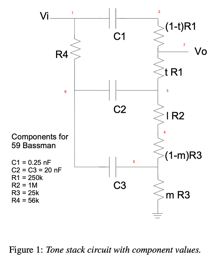
In this post we’ll be modelling one of the classic benchmark circuits - the ’59 Fender Bassman Tone Stack [1]
[1] Yeh and Smith, ‘Discretization of the ’59 Fender Bassman Tone Stack’.
2 Neutral response
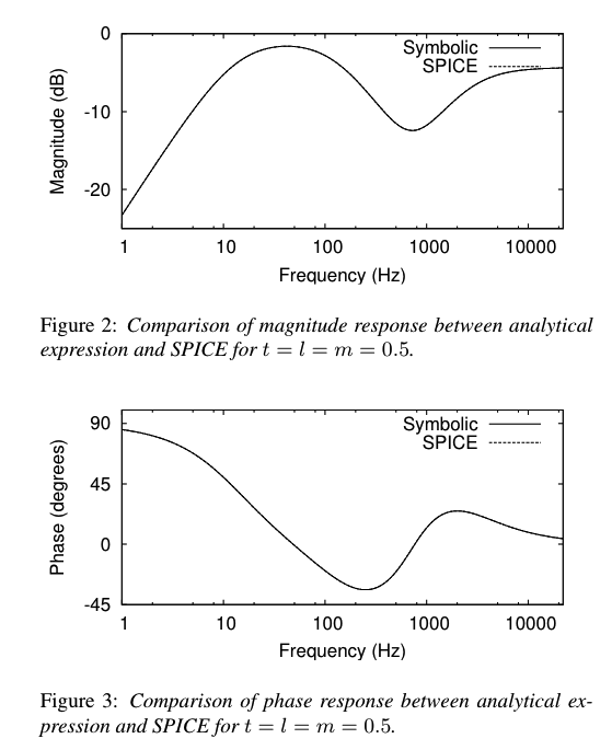
From the paper we can see that with all settings (low, mid, treble) at the midpoint, the response is far from flat. Let’s check that the MNA solution agrees:
with ModuleLoader(code_string, class_name) as m:
    fig, axs = plt.subplots(2, 1, figsize=(10, 10))
    yl, ym, yt = 0.5, 0.5, 0.5
    fig.suptitle("Amp With Netural Settings")
    f, H_dB, H, phi_deg = plot_bode(
        m, axs, args=(yl, ym, yt), label=f"l = m = t = 0.5", running_average_window=16
    )
    axs[0].set(xlim=[1, 20000], ylim=[-25, 0])
    axs[1].set(xlim=[1, 20000], ylim=[-45, 100])
    plt.tight_layout()
    plt.show()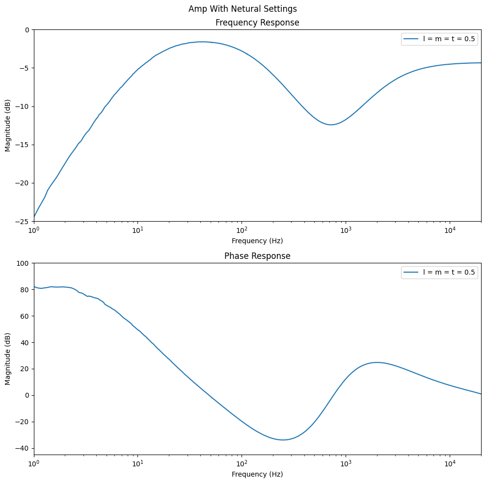
3 Varying parameters
We can also vary the low, mid and treble whilst keeping the others fixed. Note that we cannot with MNA easily reach the
import matplotlib as mpl

viridis_7 = mpl.colormaps["viridis"].resampled(7)

with ModuleLoader(code_string, class_name) as m:
    vals = [0.0625, 0.125, 0.25, 0.5, 0.75, 0.875, 0.9375]

    fig, axs = plt.subplots(3, 1, figsize=(10, 12))
    for i, yl in enumerate(vals):
        ym, yt = 0.5, 0.5
        plot_filter_response(
            m,
            axs[0],
            args=(yl, ym, yt),
            label=f"yl = {yl:.3g}",
            running_average_window=16,
            color=viridis_7.colors[i],
        )
    for i, ym in enumerate(vals):
        yl, yt = 0.5, 0.5
        plot_filter_response(
            m,
            axs[1],
            args=(yl, ym, yt),
            label=f"ym = {ym:.3g}",
            running_average_window=16,
            color=viridis_7.colors[i],
        )
    for i, yt in enumerate(vals):
        yl, ym = 0.5, 0.5
        plot_filter_response(
            m,
            axs[2],
            args=(yl, ym, yt),
            label=f"yt = {yt:.3g}",
            running_average_window=16,
            color=viridis_7.colors[i],
        )

    for i in [0, 1, 2]:
        axs[i].set(xlim=[20, None], ylim=[-20, 6])
        axs[i].legend()
    plt.tight_layout()
    plt.show()
print(code_string)
// generated with spice.hpp at 4375c34
class ToneStack {
public:
    ToneStack() : c1(2.5e-10, 0.5), c3(2e-08, 0.5), c2(2e-08, 0.5) {}

    // solution / device variables
    Capacitor c1;
    Capacitor c3;
    Capacitor c2;
    float v_1 = 0.f;
    float v_2 = 0.f;
    float v_3 = 0.f;
    float v_5 = 0.f;
    float v_6 = 0.f;
    float v_7 = 0.f;

    // dummy variable for storing stuff to expose to pybind
    float aux = 0.f;
    int iter = 0;
    auto process(float Vin, float yl, float ym, float yt, float T) {
        // constants
        const float Rpt = 250000.0;
        const float Rpm = 25000.0;
        const float R4 = 56000.0;
        const float R2 = 1000000.0;

        {
            // solution
            const float x0 = 1.0 / Rpt;
            const float x1 = yt - 1;
            const float x2 = x0 / x1;
            const float x3 = 1.0 / (c1.gc - x2);
            const float x4 = 1.0 / yt;
            const float x5 = pow(Rpt, -2);
            const float x6 = 1.0 / R2;
            const float x7 = 1.0 / yl;
            const float x8 = x6 * x7;
            const float x9 = x0 * x4;
            const float x10 = c2.gc + x8 + x9;
            const float x11 = 1.0 / x10;
            const float x12 = x5 / pow(yt, 2);
            const float x13 = ym - 1;
            const float x14 = 1.0 / Rpm;
            const float x15 = 1.0 / x13;
            const float x16 = x14 * x15;
            const float x17 = pow(R2, -2);
            const float x18 = pow(yl, -2);
            const float x19 = x17 * x18;
            const float x20 = -x11 * x19 + x16 * x8 * (-R2 * yl + Rpm * x13);
            const float x21 = 1.0 / x20;
            const float x22 = pow(x10, -2);
            const float x23 = x19 * x22;
            const float x24 = x21 * x23;
            const float x25 = 1 / (pow(Rpm, 2) * pow(x13, 2));
            const float x26 = 1.0 / (x16 * (Rpm * c3.gc * x13 * ym - 1) / ym - x21 * x25);
            const float x27 = 1.0 / R4;
            const float x28 = pow(c2.gc, 2);
            const float x29 = c2.gc * x11 * x14 * x15 * x21 * x6 * x7 - c3.gc;
            const float x30 = 1.0 / (c2.gc + c3.gc - x11 * x28 - x24 * x28 - x26 * pow(x29, 2) + x27);
            const float x31 = c2.gc * x11;
            const float x32 = c2.gc * x24;
            const float x33 = x26 * x29;
            const float x34 = x21 * x8;
            const float x35 = x16 * x34;
            const float x36 = x11 * x35 * x9;
            const float x37 = -x31 * x9 - x32 * x9 - x33 * x36;
            const float x38 = c2.ieq * x11 * x8;
            const float x39 = x16 * x21 * x38;
            const float x40 = c3.ieq - x39;
            const float x41 = -c3.ieq;
            const float x42 = x33 * x40;
            const float x43 =
                (c2.ieq * x0 * x11 * x4 + c2.ieq * x0 * x17 * x18 * x21 * x22 * x4 - x2 * x3 * (Vin * c1.gc - c1.ieq) -
                 x26 * x36 * x40 - x30 * x37 * (Vin * x27 + c2.ieq * x31 + c2.ieq * x32 - c2.ieq + x41 - x42)) /
                (-x11 * x12 - x12 * x24 - x12 * x23 * x25 * x26 / pow(x20, 2) - x2 * x4 - x30 * pow(x37, 2) - x3 * x5 / pow(x1, 2));
            const float x44 = x43 * x9;
            const float x45 =
                x30 * (Vin * x27 + c2.gc * c2.ieq * x11 + c2.gc * c2.ieq * x17 * x18 * x21 * x22 - c2.ieq - c3.ieq - x37 * x43 - x42);
            const float x46 = x11 * x44;
            const float x47 = x26 * (-x29 * x45 - x35 * x46 - x39 - x41);
            v_1 = Vin;
            v_2 = x3 * (Vin * c1.gc - c1.ieq - x2 * x43);
            v_3 = x11 * (c2.gc * x45 + c2.ieq + x34 * (-x16 * x47 + x31 * x45 * x8 + x38 + x46 * x8) + x44);
            v_5 = x47;
            v_6 = x45;
            v_7 = x43;
        }

        // state updates (caps etc)
        c1.tick(-v_1 + v_2, T);
        c3.tick(-v_5 + v_6, T);
        c2.tick(-v_3 + v_6, T);

        // outputs
        const float jout = v_7;
        return jout;
    }

    void reset() {
        c1.reset();
        c3.reset();
        c2.reset();
        v_1 = 0.f;
        v_2 = 0.f;
        v_3 = 0.f;
        v_5 = 0.f;
        v_6 = 0.f;
        v_7 = 0.f;
    }

    void calculateDC(float Vin, float yl, float ym, float yt, float T) {}
};
netlist = """
Vi 1 0 Vin
C1 1 2 C1
Pt 3 7 2 R1
R2 3 4 R2
Pm 0 5 4 R3
C3 5 6 C3
C2 3 6 C2
R4 1 6 R4
J 7 0
"""

circuit = parse_netlist(netlist, "ToneStack")
c1C, C1, c2C, C2, c3C, C3, s, Vin = symbols("c1.C C1 c2.C C2 c3.C C3 s Vin")
yl, ym, yt = symbols("yl ym yt")
Rpt, R1, Rpm, R3, R2, R4 = symbols("Rpt R1 Rpm R3 R2 R4")

numeric = {
    R1: 250000,
    R2: 100000,
    R3: 25000,
    R4: 56000,
    C1: 0.25e-9,
    C2: 20e-9,
    C3: 20e-9,
}

assumptions = {
    c1C: C1,
    c2C: C2,
    c3C: C3,
    yl: Rational(1, 2),
    ym: Rational(1, 2),
    yt: Rational(1, 2),
    Rpt: R1,
    Rpm: R3,
}

(A, x, b), component_vals_numeric = build_matrices(circuit, time_discretise=False)

# rules, (A, x, b) = run_MNA(netlist, class_name, assumptions={R2: yl*R2},
#                           method="LUsolve", simplify_sol=False, time_discretise=False)

A = simplify(A.subs(assumptions))
b = simplify(b.subs(assumptions))

display(Eq(MatMul(A, x), b))

sol_lu = A.LUsolve(b)

system = A, b
(sol,) = linsolve(system, x[:])

H = simplify(sol[6] / Vin)
display(H)n, d = fraction(H)
n = expand(n)
d = expand(d)n_c = collect(n, s)
d_c = collect(d, s)b1, b2, b3 = n_c.coeff(s, 1), n_c.coeff(s, 2), n_c.coeff(s, 3)
a0, a1, a2, a3 = d_c.coeff(s, 1), d_c.coeff(s, 1), d_c.coeff(s, 2), d_c.coeff(s, 3)
display(b1)
display(a0)simplify(b1)simplify(b1 / a0)plot(H.subs(numeric), (s, 0, 1000))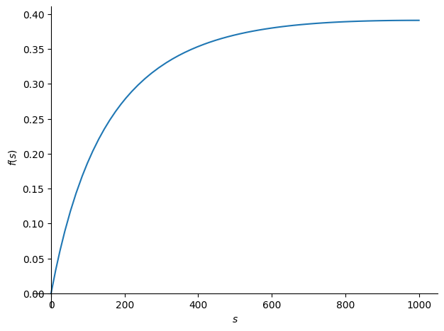
<sympy.plotting.plot.Plot at 0x155e72800>f = lambdify(s, H.subs(numeric))ss = np.geomspace(0.1, 1000)
Hs = f(ss)
plt.figure()
plt.semilogx(ss, Hs)
plt.show()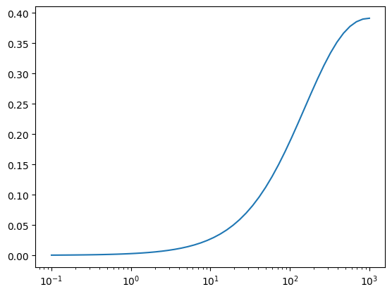
z, c = symbols("z c")
simplify(H.subs({s: c * (1 - z) / (1 + z)}))b1, b2, b3, a0, a1, a2, a3 = symbols("b1, b2, b3, a0, a1, a2, a3")
H_analytic = (b1 * s + b2 * s * s + b3 * s * s * s) / (
a0 + a1 * s + a2 * s * s + a3 * s * s * s
)
display(H_analytic)
Hz = H.subs({s: c * (1 - z) / (1 + z)})n, d = fraction(Hz)