1 Intro

In this post we’ll be working to reproduce the mki x es.edu eurorack mixer. The detailed build instructions contain lots of great information and it’s recommended to read that document first. The mixer is an ideal starting point for circuit simulation because it only contains resistors and ideal op-amps, relatively simple components to simulate. The diode clipping output stage is the most complex piece.

2 Passive Mixer

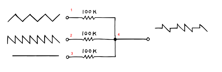
Figure 2 shows the simplest approach we can take as a mixer. This circuit simply gives you the average of the input voltages. We generalise slightly to include a third channel, and solve below using modified nodal analysis. The three input voltages are \(V1_{in}\), \(V2_{in}\), and \(V3_{in}\), and the output node (where they merge) is node 4.

netlist = """
V1 1 0 V1_in
R1 1 4 100000
V2 2 0 V2_in
R2 2 4 100000
V3 3 0 V3_in    
R3 3 4 100000    
J 4 0
"""
circuit_name = "MixerPassive"

circuit = parse_netlist(netlist, circuit_name)

(A, x, b), _, _ = solve_for_unknown_voltages_currents(circuit)
display(Eq(MatMul(A, x), b))

\(\displaystyle \left[\begin{matrix}\frac{1}{R_{1}} & 0 & 0 & - \frac{1}{R_{1}} & 1 & 0 & 0\\0 & \frac{1}{R_{2}} & 0 & - \frac{1}{R_{2}} & 0 & 1 & 0\\0 & 0 & \frac{1}{R_{3}} & - \frac{1}{R_{3}} & 0 & 0 & 1\\- \frac{1}{R_{1}} & - \frac{1}{R_{2}} & - \frac{1}{R_{3}} & \frac{1}{R_{3}} + \frac{1}{R_{2}} + \frac{1}{R_{1}} & 0 & 0 & 0\\1 & 0 & 0 & 0 & 0 & 0 & 0\\0 & 1 & 0 & 0 & 0 & 0 & 0\\0 & 0 & 1 & 0 & 0 & 0 & 0\end{matrix}\right] \left[\begin{matrix}v_{1}\\v_{2}\\v_{3}\\v_{4}\\i_{v1}\\i_{v2}\\i_{v3}\end{matrix}\right] = \left[\begin{matrix}0\\0\\0\\0\\V_{1 in}\\V_{2 in}\\V_{3 in}\end{matrix}\right]\)

Notice how each resistor contributes a characteristic “stamp” to the matrix:

\[\begin{pmatrix} 1/R_1 & -1/R_1 & \dots \\ -1/R_1 & 1/R_1 & \dots \\ \dots & \dots & \dots \end{pmatrix}\]

2.1 Kirchhoff’s Current Law

If we multiply out the matrix \(\textbf{A}\) and vector \(x\) we just get the Kirchoff balance equations at each node:

Mul(A, x)

\(\displaystyle \left[\begin{matrix}i_{v1} + \frac{v_{1}}{R_{1}} - \frac{v_{4}}{R_{1}}\\i_{v2} + \frac{v_{2}}{R_{2}} - \frac{v_{4}}{R_{2}}\\i_{v3} + \frac{v_{3}}{R_{3}} - \frac{v_{4}}{R_{3}}\\v_{4} \cdot \left(\frac{1}{R_{3}} + \frac{1}{R_{2}} + \frac{1}{R_{1}}\right) - \frac{v_{3}}{R_{3}} - \frac{v_{2}}{R_{2}} - \frac{v_{1}}{R_{1}}\\v_{1}\\v_{2}\\v_{3}\end{matrix}\right]\)

We can simplify things by assuming that the resistors are equal:

R1, R2, R3, R100k = symbols("R1, R2, R3, R_100k")
assumptions = {R1: R100k, R2: R100k, R3: R100k}

(A, x, b), solutions, _ = solve_for_unknown_voltages_currents(
    circuit, assumptions=assumptions
)
display(Eq(MatMul(A, x), b))

\(\displaystyle \left[\begin{matrix}\frac{1}{R_{100k}} & 0 & 0 & - \frac{1}{R_{100k}} & 1 & 0 & 0\\0 & \frac{1}{R_{100k}} & 0 & - \frac{1}{R_{100k}} & 0 & 1 & 0\\0 & 0 & \frac{1}{R_{100k}} & - \frac{1}{R_{100k}} & 0 & 0 & 1\\- \frac{1}{R_{100k}} & - \frac{1}{R_{100k}} & - \frac{1}{R_{100k}} & \frac{3}{R_{100k}} & 0 & 0 & 0\\1 & 0 & 0 & 0 & 0 & 0 & 0\\0 & 1 & 0 & 0 & 0 & 0 & 0\\0 & 0 & 1 & 0 & 0 & 0 & 0\end{matrix}\right] \left[\begin{matrix}v_{1}\\v_{2}\\v_{3}\\v_{4}\\i_{v1}\\i_{v2}\\i_{v3}\end{matrix}\right] = \left[\begin{matrix}0\\0\\0\\0\\V_{1 in}\\V_{2 in}\\V_{3 in}\end{matrix}\right]\)

2.2 Getting a solution

Now to obtain the output voltage we simply solve the matrix problem \(\textbf{A}x = b\) for \(x\), this gives us all unknown voltages and currents:

system = A, b
(sol,) = linsolve(system, x[:])
sol = Matrix(sol)
display(Eq(x, sol))

\(\displaystyle \left[\begin{matrix}v_{1}\\v_{2}\\v_{3}\\v_{4}\\i_{v1}\\i_{v2}\\i_{v3}\end{matrix}\right] = \left[\begin{matrix}V_{1 in}\\V_{2 in}\\V_{3 in}\\\frac{V_{1 in}}{3} + \frac{V_{2 in}}{3} + \frac{V_{3 in}}{3}\\\frac{- 2 V_{1 in} + V_{2 in} + V_{3 in}}{3 R_{100k}}\\\frac{V_{1 in} - 2 V_{2 in} + V_{3 in}}{3 R_{100k}}\\\frac{V_{1 in} + V_{2 in} - 2 V_{3 in}}{3 R_{100k}}\end{matrix}\right]\)

We’re specifically interested in the voltage at the output node, \(v_2\), which we can see is just the average of the three inputs. This is a good start, but has some serious limitations. E.g. if we only feed a voltage to the first input and have zero at \(V_{2in}\) and \(V_{3in}\), then the output volume drops by a third. We’ll address this in the Active Inverting Mixer below.

sol[3]

\(\displaystyle \frac{V_{1 in}}{3} + \frac{V_{2 in}}{3} + \frac{V_{3 in}}{3}\)

3 Active Inverting Mixer

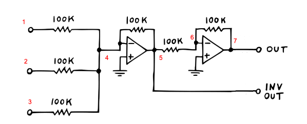
By following along with Moritz’s notes, the solution to these voltage drops is through an inverting active mixer. Note we skip the output 1K resistors as they only matter for hardware. This design outputs the (negative) sum of all inputs (without attenuation), and includes a final stage to convert that negative sum to a positive one:

# Potentiometer test
netlist = """
V1 1 0 V1_in
R_100k 1 4 100000
V2 2 0 V2_in
R_100k 2 4 100000
V3 3 0 V3_in
R_100k 3 4 100000
Oamp 0 4 5
R_100k 4 5 100000
R_100k 5 6 100000
Oamp 0 6 7
R_100k 6 7 100000
J 7 0
Jinv 5 0
"""

Rp1, Rp2, Rp3, R100k = symbols("Rp1,Rp2,Rp3,R_100k")
assumptions = {Rp1: R100k, Rp2: R100k, Rp3: R100k}
class_name = "MixerInvertingWithPots"

rules, (A, x, b) = run_MNA(
    netlist, class_name, method="LUsolve", assumptions=assumptions
)
display(Eq(MatMul(A, x), b))

\(\displaystyle \left[\begin{array}{cccccccccccc}\frac{1}{R_{100k}} & 0 & 0 & - \frac{1}{R_{100k}} & 0 & 0 & 0 & 1 & 0 & 0 & 0 & 0\\0 & \frac{1}{R_{100k}} & 0 & - \frac{1}{R_{100k}} & 0 & 0 & 0 & 0 & 1 & 0 & 0 & 0\\0 & 0 & \frac{1}{R_{100k}} & - \frac{1}{R_{100k}} & 0 & 0 & 0 & 0 & 0 & 1 & 0 & 0\\- \frac{1}{R_{100k}} & - \frac{1}{R_{100k}} & - \frac{1}{R_{100k}} & \frac{4}{R_{100k}} & - \frac{1}{R_{100k}} & 0 & 0 & 0 & 0 & 0 & 0 & 0\\0 & 0 & 0 & - \frac{1}{R_{100k}} & \frac{2}{R_{100k}} & - \frac{1}{R_{100k}} & 0 & 0 & 0 & 0 & 1 & 0\\0 & 0 & 0 & 0 & - \frac{1}{R_{100k}} & \frac{2}{R_{100k}} & - \frac{1}{R_{100k}} & 0 & 0 & 0 & 0 & 0\\0 & 0 & 0 & 0 & 0 & - \frac{1}{R_{100k}} & \frac{1}{R_{100k}} & 0 & 0 & 0 & 0 & 1\\1 & 0 & 0 & 0 & 0 & 0 & 0 & 0 & 0 & 0 & 0 & 0\\0 & 1 & 0 & 0 & 0 & 0 & 0 & 0 & 0 & 0 & 0 & 0\\0 & 0 & 1 & 0 & 0 & 0 & 0 & 0 & 0 & 0 & 0 & 0\\0 & 0 & 0 & -1 & 0 & 0 & 0 & 0 & 0 & 0 & 0 & 0\\0 & 0 & 0 & 0 & 0 & -1 & 0 & 0 & 0 & 0 & 0 & 0\end{array}\right] \left[\begin{matrix}v_{1}\\v_{2}\\v_{3}\\v_{4}\\v_{5}\\v_{6}\\v_{7}\\i_{v1}\\i_{v2}\\i_{v3}\\i_{v4}\\i_{v5}\end{matrix}\right] = \left[\begin{matrix}0\\0\\0\\0\\0\\0\\0\\V_{1 in}\\V_{2 in}\\V_{3 in}\\0\\0\end{matrix}\right]\)

Here we won’t manually solve (the SPICEWORLD library does this for us), but we’ll look at the solution at node 5 (the inverted output) and node 7 (normal output). Unlike the passive mixer, there is now no attenuation and it acts as a unity gain mixer. Specifically if we only feed a voltage to the first input and have zero at \(V2_{in}\) and \(V3_{in}\), then the output doesn’t lose any amplitude.

def show_sol(sol, index):
    display(Eq(sol[index].lhs, sol[index].rhs))


# inverted out
show_sol(rules.solutions, 5)

# inverted out
show_sol(rules.solutions, 7)

\(\displaystyle v_{5} = - V_{1 in} - V_{2 in} - V_{3 in}\)

\(\displaystyle v_{7} = V_{1 in} + V_{2 in} + V_{3 in}\)

4 Potentiometers

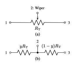
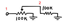
Following Holmes, ‘Potentiometer Law Modelling and Identification for Application in Physics-Based Virtual Analogue Circuits’ link, we can implement the following model of a potentiometer (or pot for short), i.e. as a pair of resistors with fraction \(y\) and \(1-y\) respectively.

As might be expected, this gives a nice linear response:

netlist = """
V0 1 0 Vin
P1 1 2 0 100000
J 2 0
"""

circuit = parse_netlist(netlist, "Potentiometer")
_, solutions, _ = solve_for_unknown_voltages_currents(circuit)

Vin, v_2, y = symbols("Vin v_2 y1")
sol_linear = simplify(solutions[v_2])
display(Eq(v_2, sol_linear))

\(\displaystyle v_{2} = Vin \left(1 - y_{1}\right)\)

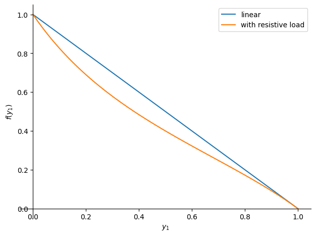
4.1 Potentiometer with resistive load.

We can test a more complex example, where there is a resistive load - as we can see this is nearly linear but now has some variation for intermediate values.

**Figure** 5: Potentiometer test circuit

netlist = """
V0 1 0 Vin
P1 1 2 0 100000
R_load 2 0 100000
J 2 0
"""

circuit = parse_netlist(netlist, "Potentiometer")
_, solutions, _ = solve_for_unknown_voltages_currents(circuit)

Vin, y, Rp1, v_2, R, RL = symbols("Vin y1 Rp1 v_2 R, R_load")

sol_with_load = simplify(solutions[v_2].subs({Rp1: R, RL: R}))
display(sol_with_load)

p1 = plot(sol_linear.subs({Vin: 1}), (y, 0, 1), show=False, label="linear", legend=True)
p2 = plot(
    sol_with_load.subs({Vin: 1}), (y, 0, 1), show=False, label="with resistive load"
)
p1.extend(p2)

p1.show()

\(\displaystyle \frac{Vin \left(y_{1} - 1\right)}{y_{1}^{2} - y_{1} - 1}\)

5 Active Inverting Mixer (with pots)

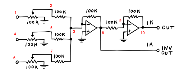
**Figure** 6: Active inverting mixer with pots

We can replace the initial resistors of the mixer in section Section 3 with pots:

netlist = """
V1 1 0 V1_in
P1 0 2 1 100000
R_100k 2 3 100000
V2 4 0 V2_in
P2 0 5 4 100000
R_100k 5 3 100000
V3 6 0 V3_in
P3 0 7 6 100000
R_100k 7 3 100000
Oamp 0 3 8
R_100k 3 8 100000
R_100k 8 9 100000
Oamp 0 9 10
R_100k 9 10 100000
J 10 0
Jinv 8 0
"""

Rp1, Rp2, Rp3, R100k = symbols("Rp1,Rp2,Rp3,R_100k")
assumptions = {Rp1: R100k, Rp2: R100k, Rp3: R100k}
class_name = "MixerInvertingWithPots"

rules, _ = run_MNA(netlist, class_name, method="LUsolve", assumptions=assumptions)

The solutions are now quite complex - focusing on the inverting output voltage, \(v_8\):

show_sol(rules.solutions, 8)

\(\displaystyle v_{8} = \frac{V_{1 in} y_{1} \left(y_{2} \left(y_{2} - 1\right) - 1\right) \left(y_{3} \left(y_{3} - 1\right) - 1\right) + V_{2 in} y_{2} \left(y_{1} \left(y_{1} - 1\right) - 1\right) \left(y_{3} \left(y_{3} - 1\right) - 1\right) + V_{3 in} y_{3} \left(y_{1} \left(y_{1} - 1\right) - 1\right) \left(y_{2} \left(y_{2} - 1\right) - 1\right)}{\left(y_{1} \left(y_{1} - 1\right) - 1\right) \left(y_{2} \left(y_{2} - 1\right) - 1\right) \left(y_{3} \left(y_{3} - 1\right) - 1\right)}\)

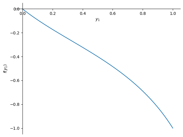
But if we e.g. zero out any 2 of the 3 inputs, it becomes simpler.

# set V2_in and V3_in to zero
V1in, V2in, V3in = symbols("V1_in, V2_in, V3_in")
simplified = rules.solutions[8].subs({V2in: 0, V3in: 0})

# display and plot
display(Eq(simplified.lhs, simplified.rhs))
_ = plot(simplified.rhs.subs({V1in: 1}), (y, 0, 1))

\(\displaystyle v_{8} = \frac{V_{1 in} y_{1}}{y_{1} \left(y_{1} - 1\right) - 1}\)

6 Putting it altogether: code generation

Finally we can convert our solution into performant C++ code. The SPICEWORLD library has a method to do this, generate_processor. As we can see, it’s not bad, but here it has failed to make a simplification for v_10, namely that R100k and x9 = 1.0 / R100k cancel. In this case we might edit the code by hand to fix the mistake.

code_string = generate_processor(rules)
print(code_string)


// generated with spice.hpp at 4375c34
class MixerInvertingWithPots {
public:
    MixerInvertingWithPots() {}

    // solution / device variables
    float v_8 = 0.f;
    float v_10 = 0.f;

    // dummy variable for storing stuff to expose to pybind
    float aux = 0.f;
    int iter = 0;
    auto process(float V1_in, float V2_in, float V3_in, float y1, float y2, float y3, float T) {
        // constants
        const float R_100k = 100000;

        {
            // solution
            const float x0 = y1 * (y1 - 1) - 1;
            const float x1 = 1.0 / x0;
            const float x2 = y2 * (y2 - 1) - 1;
            const float x3 = 1.0 / x2;
            const float x4 = y3 * (y3 - 1) - 1;
            const float x5 = 1.0 / x4;
            const float x6 = V1_in * y1;
            const float x7 = V2_in * y2;
            const float x8 = V3_in * y3;
            const float x9 = 1.0 / R_100k;
            v_8 = x1 * x3 * x5 * (x0 * x2 * x8 + x0 * x4 * x7 + x2 * x4 * x6);
            v_10 = -R_100k * (x1 * x6 * x9 + x3 * x7 * x9 + x5 * x8 * x9);
        }

        // outputs
        const float jout = v_10;
        const float jout_inv = v_8;
        return std::make_tuple(jout, jout_inv);
    }

    void reset() {
        v_8 = 0.f;
        v_10 = 0.f;
    }

    void calculateDC(float V1_in, float V2_in, float V3_in, float y1, float y2, float y3, float T) {}
};

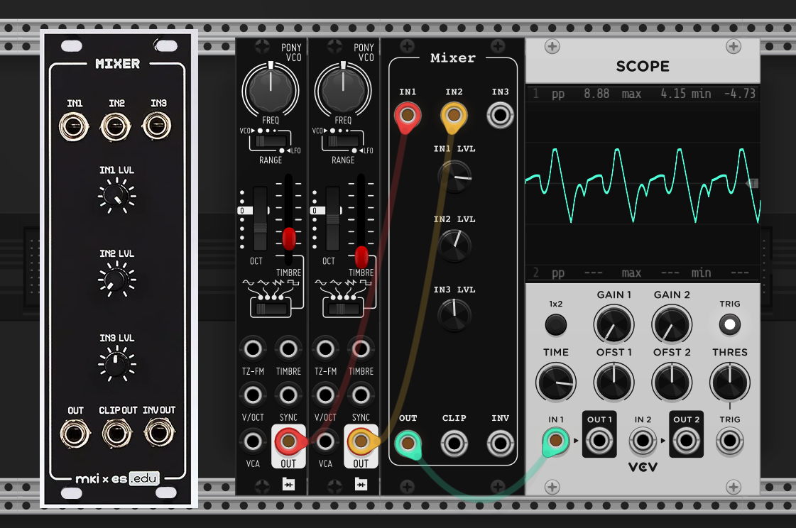
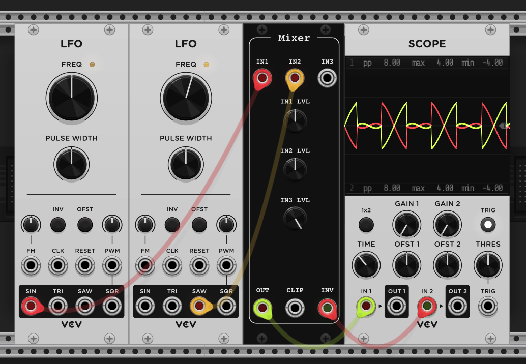
Finally we can wire up the mixer to the UI in VCV rack and have a play!

7 Diode Clipping

TBC