In this post we will explore more efficient approaches for how to solve the large matrix problems \(\textbf{M} x = b\) typically involved in circuit analysis. We focus on a nonlinear example (Schmitt Trigger), which means in practice that some entries of \(\textbf{M}\) will be changing each Newton iteration.

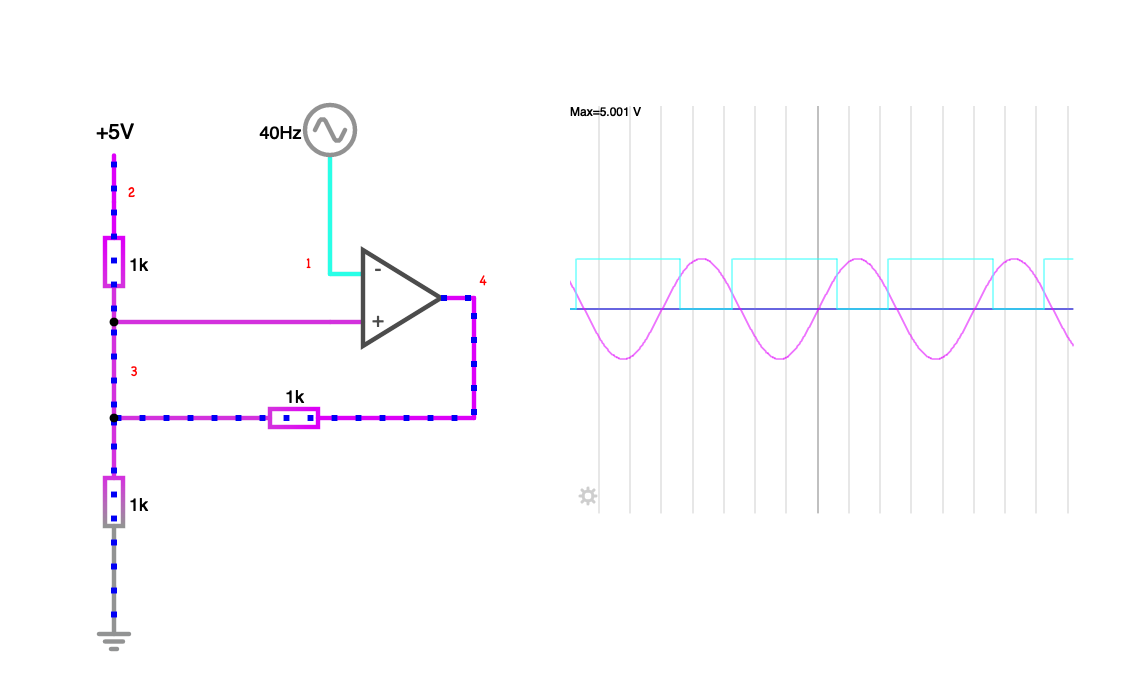
Here we’ll focus on a specific example - the Schmitt Trigger with variable thresholds. This circuit will latch and output a high voltage when the input signal goes above the high threshold \(t_{high}\), and remains so until the signal falls below a low threshold \(t_{low}\). For more details and to play around with an interactive circuit, see this Falstad example.

Code

%load_ext autoreload
%autoreload 2

Show the code

import os
import sys
import tempfile
from pathlib import Path

import numpy as np
from IPython.display import Latex, Markdown, display
from sympy import *
from sympy.codegen.ast import Assignment

module_path = os.path.abspath(os.path.join("../../.."))
if module_path not in sys.path:
    sys.path.append(module_path)

from spiceworld.circuit import parse_netlist
from spiceworld.mki_misc import generate_schmitt_thresholds
from spiceworld.solve_MNA import (
    generate_processor,
    run_MNA,
    solve_for_unknown_voltages_currents,
)

Below is a plot of the Schmitt trigger input and output signals that we will be modelling.

generate_schmitt_thresholds(plot=True)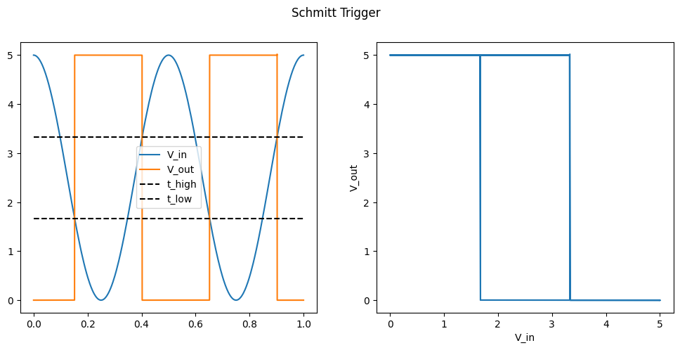

Let’s examine the example matrix problem. Note that opa.g will be updated each Newton iteration, so if solving by LU decomposition we naively will need to re-perform the full LU decomposition each iteration.

# Variable threshold Schmitt trigger
netlist = f"""
    V_in 1 0 V_in
    V_ref 2 0 5
    R1 2 3 1000
    R2 3 4 1000
    R3 3 0 1000
    OAmp 3 1 4 Vmax=5.0 Vmin=0.0
    J 4 0
    Jalt 3 0
"""

circuit = parse_netlist(netlist, "SchmittTrigger")
(M_, x_, b_), solutions, component_values = solve_for_unknown_voltages_currents(
    circuit, method="linsolve"
)
N = M_.shape[0]
display(Eq(MatMul(M_, x_), b_))

\(\displaystyle \left[\begin{matrix}0 & 0 & 0 & 0 & 1 & 0 & 0\\0 & \frac{1}{R_{1}} & - \frac{1}{R_{1}} & 0 & 0 & 1 & 0\\0 & - \frac{1}{R_{1}} & \frac{1}{R_{3}} + \frac{1}{R_{2}} + \frac{1}{R_{1}} & - \frac{1}{R_{2}} & 0 & 0 & 0\\0 & 0 & - \frac{1}{R_{2}} & \frac{1}{R_{2}} & 0 & 0 & 1\\1 & 0 & 0 & 0 & 0 & 0 & 0\\0 & 1 & 0 & 0 & 0 & 0 & 0\\- opa.g & 0 & opa.g & -1 & 0 & 0 & 0\end{matrix}\right] \left[\begin{matrix}v_{1}\\v_{2}\\v_{3}\\v_{4}\\i_{v1}\\i_{v2}\\i_{v3}\end{matrix}\right] = \left[\begin{matrix}0\\0\\0\\0\\V_{in}\\V_{ref}\\opa.Veq\end{matrix}\right]\)

Note that we are free to permute the rows of \(\textbf{M}\) (which will also require permuting for of the RHS \(b\)) and/or the cols of \(\textbf{M}\) (which will also require permuting rows of \(x\)). We can do so to move the dynamic entries of \(\textbf{M}\) (i.e. those that change every Newton iteration) to the top-left corner:

row_perms = [[0, N - 1], [1, 4]]
col_perms = [[1, 2]]

M = M_.permute(row_perms, orientation="rows").permute(col_perms, orientation="cols")
x = x_.permute(col_perms, orientation="rows")
b = b_.permute(row_perms, orientation="rows")

display(Eq(MatMul(M, x), b))

\(\displaystyle \left[\begin{matrix}- opa.g & opa.g & 0 & -1 & 0 & 0 & 0\\1 & 0 & 0 & 0 & 0 & 0 & 0\\0 & \frac{1}{R_{3}} + \frac{1}{R_{2}} + \frac{1}{R_{1}} & - \frac{1}{R_{1}} & - \frac{1}{R_{2}} & 0 & 0 & 0\\0 & - \frac{1}{R_{2}} & 0 & \frac{1}{R_{2}} & 0 & 0 & 1\\0 & - \frac{1}{R_{1}} & \frac{1}{R_{1}} & 0 & 0 & 1 & 0\\0 & 0 & 1 & 0 & 0 & 0 & 0\\0 & 0 & 0 & 0 & 1 & 0 & 0\end{matrix}\right] \left[\begin{matrix}v_{1}\\v_{3}\\v_{2}\\v_{4}\\i_{v1}\\i_{v2}\\i_{v3}\end{matrix}\right] = \left[\begin{matrix}opa.Veq\\V_{in}\\0\\0\\0\\V_{ref}\\0\end{matrix}\right]\)

We can now partition the permuted matrix problem into a block matrix:

Show the code

def submatrix():
    m, n = symbols("m n")

    M__ = MatrixSymbol("M", n + m, n + m)

    A_ = MatrixSymbol("A", n, n)
    B_ = MatrixSymbol("B", n, m)
    C_ = MatrixSymbol("C", m, n)
    D_ = MatrixSymbol("D", m, m)
    lhs = BlockMatrix([[A_, B_], [C_, D_]])
    display(Eq(M__, lhs))


submatrix()

\(\displaystyle M = \left[\begin{matrix}A & B\\C & D\end{matrix}\right]\)

After partitioning, the problem now looks like this:

q = 2
A = M[0:q, 0:q]
B = M[0:q, q:]
C = M[q:, 0:q]
D = M[q:, q:]

x1, x2 = Matrix(x[0:q]), Matrix(x[q:])
b1, b2 = Matrix(b[0:q]), Matrix(b[q:])

rhs = BlockMatrix([[A, B], [C, D]])
display(Eq(MatMul(rhs, BlockMatrix([[x1], [x2]])), BlockMatrix([[b1], [b2]])))

\(\displaystyle \left[\begin{matrix}\left[\begin{matrix}- opa.g & opa.g\\1 & 0\end{matrix}\right] & \left[\begin{matrix}0 & -1 & 0 & 0 & 0\\0 & 0 & 0 & 0 & 0\end{matrix}\right]\\\left[\begin{matrix}0 & \frac{1}{R_{3}} + \frac{1}{R_{2}} + \frac{1}{R_{1}}\\0 & - \frac{1}{R_{2}}\\0 & - \frac{1}{R_{1}}\\0 & 0\\0 & 0\end{matrix}\right] & \left[\begin{matrix}- \frac{1}{R_{1}} & - \frac{1}{R_{2}} & 0 & 0 & 0\\0 & \frac{1}{R_{2}} & 0 & 0 & 1\\\frac{1}{R_{1}} & 0 & 0 & 1 & 0\\1 & 0 & 0 & 0 & 0\\0 & 0 & 1 & 0 & 0\end{matrix}\right]\end{matrix}\right] \left[\begin{matrix}\left[\begin{matrix}v_{1}\\v_{3}\end{matrix}\right]\\\left[\begin{matrix}v_{2}\\v_{4}\\i_{v1}\\i_{v2}\\i_{v3}\end{matrix}\right]\end{matrix}\right] = \left[\begin{matrix}\left[\begin{matrix}opa.Veq\\V_{in}\end{matrix}\right]\\\left[\begin{matrix}0\\0\\0\\V_{ref}\\0\end{matrix}\right]\end{matrix}\right]\)

Then, assuming that the subproblems remain solvable, we can then solve as follows, noting that the second step uses the solutions from the first on the RHS:

assert D.det() != 0
assert (A - B * D.inv() * C).det() != 0

display(Eq(MatMul(A - B * D.inv() * C, x1), b1))
display(Eq(MatMul(D, x2), b2 - C * x1))

\(\displaystyle \left[\begin{matrix}- opa.g & - R_{2} \cdot \left(\frac{1}{R_{3}} + \frac{1}{R_{2}} + \frac{1}{R_{1}}\right) + opa.g\\1 & 0\end{matrix}\right] \left[\begin{matrix}v_{1}\\v_{3}\end{matrix}\right] = \left[\begin{matrix}opa.Veq\\V_{in}\end{matrix}\right]\)

\(\displaystyle \left[\begin{matrix}- \frac{1}{R_{1}} & - \frac{1}{R_{2}} & 0 & 0 & 0\\0 & \frac{1}{R_{2}} & 0 & 0 & 1\\\frac{1}{R_{1}} & 0 & 0 & 1 & 0\\1 & 0 & 0 & 0 & 0\\0 & 0 & 1 & 0 & 0\end{matrix}\right] \left[\begin{matrix}v_{2}\\v_{4}\\i_{v1}\\i_{v2}\\i_{v3}\end{matrix}\right] = \left[\begin{matrix}- v_{3} \cdot \left(\frac{1}{R_{3}} + \frac{1}{R_{2}} + \frac{1}{R_{1}}\right)\\\frac{v_{3}}{R_{2}}\\\frac{v_{3}}{R_{1}}\\V_{ref}\\0\end{matrix}\right]\)

We can go ahead and solve this. The LHS entries of the first matrix problem will be changing each iteration, but is now just 2x2 in size so the impact is minimal. Then a second larger but constant matrix problem is solved where only the RHS updates. Whilst you shouldn’t/wouldn’t typically solve these \(\textbf{A}x = b\) problems by explicitly inverting \(\textbf{A}\), you can see that if you did, the first is easy to invert each iteration and the second can be inverted once at program start.

Here we can finish the calculation symbolically but that may not always be practical for bigger systems. Note that the solution for the second set of voltages/currents depends on the first (i.e. \(v_1\) and \(v_3\)).

system = (A - B * D.inv() * C), b1 - B * D.inv() * b2
(sol_x1,) = linsolve(system, x1[:])
sol_x1 = Matrix(simplify(sol_x1))
display(Eq(x1, sol_x1))

system = D, b2 - C * x1
(sol_x2,) = linsolve(system, x2[:])
sol_x2 = Matrix(simplify(sol_x2))
display(Eq(x2, sol_x2))

\(\displaystyle \left[\begin{matrix}v_{1}\\v_{3}\end{matrix}\right] = \left[\begin{matrix}V_{in}\\\frac{- R_{1} R_{3} V_{in} opa.g - R_{1} R_{3} opa.Veq + R_{2} R_{3} V_{ref}}{R_{1} R_{2} - R_{1} R_{3} opa.g + R_{1} R_{3} + R_{2} R_{3}}\end{matrix}\right]\)

\(\displaystyle \left[\begin{matrix}v_{2}\\v_{4}\\i_{v1}\\i_{v2}\\i_{v3}\end{matrix}\right] = \left[\begin{matrix}V_{ref}\\\frac{R_{1} R_{2} v_{3} + R_{1} R_{3} v_{3} - R_{2} R_{3} V_{ref} + R_{2} R_{3} v_{3}}{R_{1} R_{3}}\\0\\\frac{- V_{ref} + v_{3}}{R_{1}}\\\frac{- R_{1} v_{3} + R_{3} V_{ref} - R_{3} v_{3}}{R_{1} R_{3}}\end{matrix}\right]\)

Finally we can check that the solution matches that of the naive single matrix problem:

# just a little cleaner for visualisation
op_pre_g, op_post_g, op_pre_V, op_post_V = symbols("opa.g g_op opa.Veq V_eq")
subs = {op_pre_g: op_post_g, op_pre_V: op_post_V}

sol = Matrix([sol_x1, sol_x2])
permuted_sol = {l: simplify(r) for l, r in zip(x, sol)}
permuted_sol = {l: r.subs(permuted_sol) for l, r in zip(x, sol)}

for i, variable in enumerate(solutions.keys()):
    if str(variable) == "v_0":
        # skip ground
        continue

    display(Eq(variable, simplify(permuted_sol[variable].subs(subs))))

    assert simplify(solutions[variable] - permuted_sol[variable]) == 0

\(\displaystyle v_{1} = V_{in}\)

\(\displaystyle v_{2} = V_{ref}\)

\(\displaystyle v_{3} = \frac{R_{3} \left(- R_{1} V_{eq} - R_{1} V_{in} g_{op} + R_{2} V_{ref}\right)}{R_{1} R_{2} - R_{1} R_{3} g_{op} + R_{1} R_{3} + R_{2} R_{3}}\)

\(\displaystyle v_{4} = \frac{- R_{1} R_{2} V_{eq} - R_{1} R_{2} V_{in} g_{op} - R_{1} R_{3} V_{eq} - R_{1} R_{3} V_{in} g_{op} - R_{2} R_{3} V_{eq} - R_{2} R_{3} V_{in} g_{op} + R_{2} R_{3} V_{ref} g_{op}}{R_{1} R_{2} - R_{1} R_{3} g_{op} + R_{1} R_{3} + R_{2} R_{3}}\)

\(\displaystyle i_{v1} = 0\)

\(\displaystyle i_{v2} = \frac{- R_{2} V_{ref} - R_{3} V_{eq} - R_{3} V_{in} g_{op} + R_{3} V_{ref} g_{op} - R_{3} V_{ref}}{R_{1} R_{2} - R_{1} R_{3} g_{op} + R_{1} R_{3} + R_{2} R_{3}}\)

\(\displaystyle i_{v3} = \frac{R_{1} V_{eq} + R_{1} V_{in} g_{op} + R_{3} V_{eq} + R_{3} V_{in} g_{op} - R_{3} V_{ref} g_{op} + R_{3} V_{ref}}{R_{1} R_{2} - R_{1} R_{3} g_{op} + R_{1} R_{3} + R_{2} R_{3}}\)

We can abuse the code gen to show the diffence between the naive and optimised approachs:

rules, _ = run_MNA(netlist, "SchmittTrigger", method="linsolve")
code_string = generate_processor(rules)
display(Markdown("# Naive approach"))
print(code_string)

rules.solutions = [Assignment(l, r) for l, r in zip(x1, sol_x1)]
rules.state_updates += [
    ccode(Assignment(l, r)) for l, r in zip(x2, sol_x2) if str(l).startswith("v_")
]

code_string = generate_processor(rules)
display(Markdown("# Optimised approach"))
print(code_string)

Naive approach


// generated with spice.hpp at 4375c34
class SchmittTrigger {
public:
    SchmittTrigger() : opa(5.0, 0.0) {}

    // solution / device variables
    OpAmp opa;
    float v_1 = 0.f, v_1_prev = 0.f;
    float v_3 = 0.f, v_3_prev = 0.f;
    float v_4 = 0.f, v_4_prev = 0.f;

    // dummy variable for storing stuff to expose to pybind
    float aux = 0.f;
    int iter = 0;
    auto process(float V_in, float T) {
        // constants
        const float V_ref = 5.0;
        const float R1 = 1000;
        const float R2 = 1000;
        const float R3 = 1000;

        for (iter = 0; iter < MAX_ITER; ++iter) {
            // solution
            const float x0 = V_in * opa.g;
            const float x1 = R1 * R2;
            const float x2 = R1 * R3;
            const float x3 = R2 * R3;
            const float x4 = opa.g * x2;
            const float x5 = 1.0 / (x1 + x2 + x3 - x4);
            v_1 = V_in;
            v_3 = R3 * x5 * (-R1 * opa.Veq - R1 * x0 + R2 * V_ref);
            v_4 = x5 * (R2 * R3 * V_ref * opa.g - V_in * x4 - opa.Veq * x1 - opa.Veq * x2 - opa.Veq * x3 - x0 * x1 - x0 * x3);

            // linearisation / newton
            opa.newton(v_3, v_1);

            // convergence check
            bool converged = true;
            converged = converged & (std::abs(v_1 - v_1_prev) < EPS);
            converged = converged & (std::abs(v_3 - v_3_prev) < EPS);
            converged = converged & (std::abs(v_4 - v_4_prev) < EPS);
            if (converged) {
                break;
            }
            v_1_prev = v_1;
            v_3_prev = v_3;
            v_4_prev = v_4;
        }

        // outputs
        const float jout = v_4;
        const float jout_alt = v_3;
        return std::make_tuple(jout, jout_alt);
    }

    void reset() {
        v_1 = v_1_prev = 0.f;
        v_3 = v_3_prev = 0.f;
        v_4 = v_4_prev = 0.f;
    }

    void calculateDC(float V_in, float T) {}
};


// generated with spice.hpp at 4375c34
class SchmittTrigger {
public:
    SchmittTrigger() : opa(5.0, 0.0) {}

    // solution / device variables
    OpAmp opa;
    float v_1 = 0.f, v_1_prev = 0.f;
    float v_3 = 0.f, v_3_prev = 0.f;
    float v_4 = 0.f, v_4_prev = 0.f;
    float v_1 = 0.f, v_1_prev = 0.f;
    float v_3 = 0.f, v_3_prev = 0.f;

    // dummy variable for storing stuff to expose to pybind
    float aux = 0.f;
    int iter = 0;
    auto process(float V_in, float T) {
        // constants
        const float V_ref = 5.0;
        const float R1 = 1000;
        const float R2 = 1000;
        const float R3 = 1000;

        for (iter = 0; iter < MAX_ITER; ++iter) {
            // solution
            const float x0 = R1 * R3;
            const float x1 = opa.g * x0;
            v_1 = V_in;
            v_3 = (R2 * R3 * V_ref - V_in * x1 - opa.Veq * x0) / (R1 * R2 + R2 * R3 + x0 - x1);

            // linearisation / newton
            opa.newton(v_3, v_1);

            // convergence check
            bool converged = true;
            converged = converged & (std::abs(v_1 - v_1_prev) < EPS);
            converged = converged & (std::abs(v_3 - v_3_prev) < EPS);
            if (converged) {
                break;
            }
            v_1_prev = v_1;
            v_3_prev = v_3;
        }

        // state updates (caps etc)
        v_2 = V_ref;
        v_4 = (R1 * R2 * v_3 + R1 * R3 * v_3 - R2 * R3 * V_ref + R2 * R3 * v_3) / (R1 * R3);

        // outputs
        const float jout = v_4;
        const float jout_alt = v_3;
        return std::make_tuple(jout, jout_alt);
    }

    void reset() {
        v_1 = v_1_prev = 0.f;
        v_3 = v_3_prev = 0.f;
    }

    void calculateDC(float V_in, float T) {}
};